The Nonprofit Sector in Brief

The Nonprofit Sector in Brief 2019

6.4.2020

NCCS Team

The Nonprofit Sector in Brief 2019

by NCCS Project Team
June 2020

This brief discusses trends in the number and finances of 501(c)(3) public charities and key data insights on important resources for the nonprofit sector, such as: private charitable contributions and grantmaking by foundations.

Highlights

Approximately 1.54 million nonprofits were registered with the Internal Revenue Service (IRS) in 2016, an increase of 4.5 percent from 2006.
The nonprofit sector contributed an estimated $1.047.2 trillion to the US economy in 2016, composing 5.6 percent of the country's gross domestic product (GDP).¹
Of the nonprofit organizations registered with the IRS, 501(c)(3) public charities accounted for just over three-quarters of revenue and expenses for the nonprofit sector as a whole ($2.04 trillion and $1.94 trillion, respectively) and just under two-thirds of the nonprofit sector's total assets ($3.79 trillion).
In 2018, total private giving from individuals, foundations, and businesses totaled $427.71 billion (Giving USA Foundation 2019), a decrease of -1.7 percent from 2017 (after adjusting for inflation). According to Giving USA (2018) total charitable giving rose for consecutive years from 2014 to 2017, making 2017 the largest single year for private charitable giving, even after adjusting for inflation.
An estimated 25.1 percent of US adults volunteered in 2017, contributing an estimated 8.8 billion hours. This is a 1.6 percent increase from 2016. The value of these hours is approximately $195.0 billion.

Size and Scope of the Nonprofit Sector

#Define Table 1 Function
Table1 <- function(datayear) {
 
  ###
  #Step1: Pull from raw bmf data to get Number of registered organizations
  ###
 
  #Step1a: Create function to pull in BMF data
  byear <- function(datayear) {
 
    #get BMF file names:
    bmf1 <- as.character(paste("bmf", (datayear -10), sep =""))
    bmf2 <- as.character(paste("bmf", (datayear -5), sep =""))
    bmf3 <- as.character(paste("bmf", (datayear), sep =""))
 
    #for each BMF file name, run the following:
    bcomponent <- function(bmfnum, year_of_int){
 
      #get dataset  
      bmf <- get(bmfnum)
 
      #calculate all registered nonprofits
      all <- bmf %>%
        filter((OUTNCCS != "OUT")) %>%
        summarize(
          year = as.character(year_of_int),
          "All registered nonprofits" = n()
        ) 
 
      #calculate all public charities
      pc <- bmf %>%  
        filter((FNDNCD != "02" & FNDNCD!= "03" & FNDNCD != "04"), (SUBSECCD == "03"|SUBSECCD== "3"), (OUTNCCS != "OUT")) %>%
        summarize(
          year = as.character(year_of_int),
          "501(c)(3) public charities" = n()
        )
 
      #combine registered nonprofits and public charities
      combined <- all %>%
        left_join(pc, by = "year")
 
      #return combined file
      return(combined)
    }
 
    #run function for each year
    bcomp1 <-bcomponent(bmf1, (datayear -10))
    bcomp2 <-bcomponent(bmf2, (datayear -5))
    bcomp3 <-bcomponent(bmf3, datayear)
 
    #merge years
    total <- rbind(bcomp1, bcomp2, bcomp3)
 
    #return final
    return(total)
  }
 
  #Step 1b: run against year of interest:
  btest<- byear(datayear)
 
  ###
  #Step 2: pull correct core file years
  ###
 
  #Step 2a: function to pull correct years starting from base year:
  T1grab = function(yr) {
    output <- c(yr-10, 
                yr-5, 
                yr)
    return(list(output))
  }
 
  #Step 2b: pull the right years:
  T1years <-T1grab(datayear)
 
  #Step 2c: Function for individual years of core files
 
  T1Fin<-  function(datayear) {
 
    pcname <- as.character(paste("core", datayear, "pc", sep =""))
    coname <- as.character(paste("core", datayear, "co", sep =""))
    pfname <- as.character(paste("core", datayear, "pf", sep =""))
 
    pcfile <- get(pcname)
    cofile <- get(coname)
    pffile <- get(pfname)
 
    pcfile <- if(datayear < 2010) filter(pcfile, (GRREC >= 25000)) else filter(pcfile, ((GRREC >= 50000)|(TOTREV>50000)))
    cofile <- if(datayear < 2010) filter(cofile, ((GRREC >= 25000)|(TOTREV>25000))) else filter(cofile, ((GRREC >= 50000)|(TOTREV>50000)))
 
    pc <-pcfile %>%
      filter((is.na(OUTNCCS)|OUTNCCS != "OUT"), (FNDNCD != "02" & FNDNCD!= "03" & FNDNCD != "04")) %>%
      summarize(
        Reporting = n(),
        "Revenue ($ billions)" = round((sum(as.numeric(TOTREV), na.rm =TRUE))/1000000000, digits =2),
        "Expenses ($ billions)" = round((sum(as.numeric(EXPS), na.rm =TRUE))/1000000000, digits =2),
        "Assets ($ billions)" = round((sum(as.numeric(ASS_EOY), na.rm =TRUE))/1000000000, digits=2))
    pc <- melt(pc)
    colnames(pc)[2] <- "PC"
 
    co <- cofile %>%
      filter((OUTNCCS != "OUT")) %>%
      summarize(
        Reporting = n(),
        "Revenue ($ billions)" = round((sum(as.numeric(TOTREV), na.rm =TRUE))/1000000000, digits =2),
        "Expenses ($ billions)" = round((sum(as.numeric(EXPS), na.rm =TRUE))/1000000000, digits =2),
        "Assets ($ billions)" = round((sum(as.numeric(ASS_EOY), na.rm =TRUE))/1000000000, digits=2))
    co <- melt(co)
    colnames(co)[2] <- "CO"
 
    pf <- pffile %>%
      filter(OUTNCCS != "OUT") %>%
      summarize(
        Reporting = n(),
        "Revenue ($ billions)" = round((sum(as.numeric(P1TOTREV), na.rm =TRUE))/1000000000, digits =2),
        "Expenses ($ billions)" = round((sum(as.numeric(P1TOTEXP), na.rm =TRUE))/1000000000, digits =2),
        "Assets ($ billions)" = round((sum(as.numeric(P2TOTAST), na.rm =TRUE))/1000000000, digits=2))
    pf <- melt(pf)
    colnames(pf)[2] <- "PF"
 
    Table1 <- pc %>%
      left_join(co, by = "variable") %>%
      left_join(pf, by = "variable") %>%
      transmute(
        variable = variable,
        "Reporting nonprofits" = (PC+CO+PF),
        "Reporting public charities" = PC)
    Table1 <- melt(Table1)
    colnames(Table1)[2]= "Type"
    colnames(Table1)[3]= as.character(datayear)
    Table1$variable <-ifelse(Table1$variable == "Reporting" & Table1$Type == "Reporting nonprofits", 
                             "Reporting nonprofits", as.character(Table1$variable))
    Table1$variable <-ifelse(Table1$variable == "Reporting" & Table1$Type == "Reporting public charities", 
                             "Reporting public charities", as.character(Table1$variable))
    return(Table1)
  }
 
  #Step 2d: run core file function for each core file year:
  comp1 <- T1Fin(T1years[[1]][1])
  comp2 <- T1Fin(T1years[[1]][2])
  comp3 <- T1Fin(T1years[[1]][3])
 
  #Step 2e: join multiple core file years together
  Table1All <- comp1 %>%
    left_join(comp2, by = c("Type", "variable")) %>%
    left_join(comp3, by = c("Type", "variable")) 
 
  #Step 2f: drop intermediary column
  Table1All <- Table1All[-2]
 
  ###
  #Step 3 Merge with BMF data
  ###
 
  AllRegNonprofits<- data.frame("All registered nonprofits", btest[[2]][1], btest[[2]][2], btest[[2]][3])
  names(AllRegNonprofits) <- names(Table1All)
  AllPCs<- data.frame("501(c)(3) public charities", btest[[3]][1], btest[[3]][2], btest[[3]][3])
  names(AllPCs) <- names(Table1All)
 
  Table1All <- rbind(Table1All, AllRegNonprofits, AllPCs)
 
  ###
  #Step 4: Calculate change over time
  ###
  Table1All <- Table1All %>%
    mutate(
      ChangeA = round(((Table1All[, as.character(datayear-5)] - Table1All[, as.character(datayear-10)])/(Table1All[, as.character(datayear-10)]))
                      *100, digits=1),
      ChangeB = round(((Table1All[, as.character(datayear)] - Table1All[, as.character(datayear-10)])/(Table1All[, as.character(datayear-10)]))
                      *100, digits=1)
    )
 
  ###
  #Step 5: calculate inflation adjustments
  ###
  Table1All <- Table1All %>%
    mutate(
      Y1 = round(((Table1All[, as.character(datayear-10)] * inflindex[as.character(datayear),])/(inflindex[as.character(datayear-10),])), digits=3),
      Y2 = round(((Table1All[, as.character(datayear-5)] * inflindex[as.character(datayear),])/(inflindex[as.character(datayear-5),])), digits=3),
      Y3 = round(((Table1All[, as.character(datayear)] * inflindex[as.character(datayear),])/(inflindex[as.character(datayear),])), digits=3),
      ChangeAInfl = round(((Y2-Y1)/Y1)*100, digits = 1),
      ChangeBInfl = round(((Y3-Y1)/Y1)*100, digits = 1)
    )
 
  ###
  #Step 6: Format and prepare final table
  ###
 
  #Step 6a: remove intermediary columns
  Table1All[7:9] <- list(NULL)
 
  #Step 6b: reorder columns to fit Nonprofit Sector in Brief
  Table1All <- Table1All[, c(1,2,3,5,7,4,6,8)]
 
  #Step 6c: omit numerical count columns from inflation adjustments
  Table1All[[5]][1] <- "--"
  Table1All[[5]][5] <- "--"
  Table1All[[8]][1] <- "--"
  Table1All[[8]][5] <- "--"
  Table1All[[5]][9] <- "--"
  Table1All[[5]][10] <- "--"
  Table1All[[8]][9] <- "--"
  Table1All[[8]][10] <- "--"
 
  #Step 6d: rename columns
  colnames(Table1All)[1] <- ""
  colnames(Table1All)[4] <- paste("% change, ", as.character(datayear -10), "\u2013", as.character(datayear - 5), sep = "")
  colnames(Table1All)[5] <- paste("% change, ", as.character(datayear -10), "\u2013", as.character(datayear - 5), " (inflation adjusted)", sep = "")
  colnames(Table1All)[7] <- paste("% change, ", as.character(datayear -10), "\u2013", as.character(datayear ), sep = "")
  colnames(Table1All)[8] <- paste("% change, ", as.character(datayear -10), "\u2013", as.character(datayear ), " (inflation adjusted)", sep = "")
 
  #Step6e: reorder rows
  Table1All <- Table1All[c(9,1,2,3,4,10,5,6,7,8),]
 
  #Step 6f: return final output
  return(Table1All)
}
 
#Create Table 1 based on 2015 data
Table1_2016 <-Table1(params$NCCSDataYr)
write.csv(Table1_2016, "Tables/NSiB_Table1.csv")
 
 
 
#Define Table 1 Current Growth Function (Appendix Table Showing only most recent growth)
Table1CurGrowth <- function(datayear) {
  ###
  #Step1: Pull from raw BMF data to get Number of registered organizations
  ###
 
  #Step1a: Create function
  byear <- function(datayear) {
 
    #get BMF file names:
    bmf1 <- as.character(paste("bmf", (datayear -1), sep =""))
    bmf2 <- as.character(paste("bmf", (datayear), sep =""))
 
    #for each BMF file name, run the following:
    bcomponent <- function(bmfnum, year_of_int){
 
      #get dataset  
      bmf <- get(bmfnum)
 
      #calculate all registered nonprofits
      all <- bmf %>%
        filter((OUTNCCS != "OUT")) %>%
        summarize(
          year = as.character(year_of_int),
          "All registered nonprofits" = n()
        ) 
 
      #calculate all public charities
      pc <- bmf %>%  
        filter((FNDNCD != "02" & FNDNCD!= "03" & FNDNCD != "04"), (SUBSECCD == "03"|SUBSECCD== "3"), (OUTNCCS != "OUT")) %>%
        summarize(
          year = as.character(year_of_int),
          "501(c)(3) public charities" = n()
        )
 
      #combine registered nonprofits and public charities
      combined <- all %>%
        left_join(pc, by = "year")
 
      #return combined file
      return(combined)
    }
 
    #run function for each year
    bcomp1 <-bcomponent(bmf1, (datayear -1))
    bcomp2 <-bcomponent(bmf2, (datayear))
 
    #merge years
    total <- rbind(bcomp1, bcomp2)
 
    #return final
    return(total)
  }
 
  #Step 1b: run against year of interest:
  btest<- byear(datayear) 
 
  ###
  #Step 2: Pull NCCS Core File data
  ###
 
  #Step 2a: function to pull correct years starting from base year:
  T1grab = function(yr) {
    output <- c(yr-1, 
                yr)
    return(list(output))
  }
 
  #Step 2b: pull the right years:
  T1years <-T1grab(datayear)  
 
  #Step 2c: Function for individual years of core files
 
  T1Fin<-  function(datayear) {  
 
    pcname <- as.character(paste("core", datayear, "pc", sep =""))
    coname <- as.character(paste("core", datayear, "co", sep =""))
    pfname <- as.character(paste("core", datayear, "pf", sep =""))
 
    pcfile <- get(pcname)
    cofile <- get(coname)
    pffile <- get(pfname)
 
    pcfile <- if(datayear < 2010) filter(pcfile, (GRREC >= 25000)) else filter(pcfile, ((GRREC >= 50000)|(TOTREV>50000)))
    cofile <- if(datayear < 2010) filter(cofile, ((GRREC >= 25000)|(TOTREV>25000))) else filter(cofile, ((GRREC >= 50000)|(TOTREV>50000)))
 
    pc <-pcfile %>%
      filter((is.na(OUTNCCS)|OUTNCCS != "OUT"), (FNDNCD != "02" & FNDNCD!= "03" & FNDNCD != "04")) %>%
      summarize(
        Reporting = n(),
        "Revenue ($ billions)" = round((sum(as.numeric(TOTREV), na.rm =TRUE))/1000000000, digits =2),
        "Expenses ($ billions)" = round((sum(as.numeric(EXPS), na.rm =TRUE))/1000000000, digits =2),
        "Assets ($ billions)" = round((sum(as.numeric(ASS_EOY), na.rm =TRUE))/1000000000, digits=2))
    pc <- melt(pc)
    colnames(pc)[2] <- "PC"
 
    co <- cofile %>%
      filter((OUTNCCS != "OUT")) %>%
      summarize(
        Reporting = n(),
        "Revenue ($ billions)" = round((sum(as.numeric(TOTREV), na.rm =TRUE))/1000000000, digits =2),
        "Expenses ($ billions)" = round((sum(as.numeric(EXPS), na.rm =TRUE))/1000000000, digits =2),
        "Assets ($ billions)" = round((sum(as.numeric(ASS_EOY), na.rm =TRUE))/1000000000, digits=2))
    co <- melt(co)
    colnames(co)[2] <- "CO"
 
    pf <- pffile %>%
      filter(OUTNCCS != "OUT") %>%
      summarize(
        Reporting = n(),
        "Revenue ($ billions)" = round((sum(as.numeric(P1TOTREV), na.rm =TRUE))/1000000000, digits =2),
        "Expenses ($ billions)" = round((sum(as.numeric(P1TOTEXP), na.rm =TRUE))/1000000000, digits =2),
        "Assets ($ billions)" = round((sum(as.numeric(P2TOTAST), na.rm =TRUE))/1000000000, digits=2))
    pf <- melt(pf)
    colnames(pf)[2] <- "PF"
 
    Table1 <- pc %>%
      left_join(co, by = "variable") %>%
      left_join(pf, by = "variable") %>%
      transmute(
        variable = variable,
        "Reporting nonprofits" = (PC+CO+PF),
        "Reporting public charities" = PC)
    Table1 <- melt(Table1)
    colnames(Table1)[2]= "Type"
    colnames(Table1)[3]= as.character(datayear)
    Table1$variable <-ifelse(Table1$variable == "Reporting" & Table1$Type == "Reporting nonprofits", 
                             "Reporting nonprofits", as.character(Table1$variable))
    Table1$variable <-ifelse(Table1$variable == "Reporting" & Table1$Type == "Reporting public charities", 
                             "Reporting public charities", as.character(Table1$variable))
    return(Table1)
  }
 
  #Step 2d: run core file function for each core file year:
  comp1 <- T1Fin(T1years[[1]][1])
  comp2 <- T1Fin(T1years[[1]][2])
 
  #Setp 2e: join multiple core file years together
  Table1CG <- comp1 %>%
    left_join(comp2, by = c("Type", "variable"))
 
  #Step 2f: drop intermediary column
  Table1CG <- Table1CG[-2]
 
  ####
  #Step 3: Merge with BMF data
  ###
 
  AllRegNonprofits<- data.frame("All registered nonprofits", btest[[2]][1], btest[[2]][2])
  names(AllRegNonprofits) <- names(Table1CG)
  AllPCs<- data.frame("501(c)(3) public charities", btest[[3]][1], btest[[3]][2])
  names(AllPCs) <- names(Table1CG)
 
  Table1CG <- rbind(Table1CG, AllRegNonprofits, AllPCs)
 
  ###
  #Step 4: Calculate change over time
  ###
  Table1CG <- Table1CG %>%
    mutate(
      Change = round(((Table1CG[, as.character(datayear)] - Table1CG[, as.character(datayear-1)])/(Table1CG[, as.character(datayear-1)]))
                      *100, digits=1)
    )  
 
  ###
  #Step 5: calculate inflation adjustments
  ###
  Table1CG <- Table1CG %>%
    mutate(
      Y1_InflAdj = round(((Table1CG[, as.character(datayear-1)] * inflindex[as.character(datayear),])/(inflindex[as.character(datayear-1),])), digits=3),  
      Y2_InflAdj = round(((Table1CG[, as.character(datayear)] * inflindex[as.character(datayear),])/(inflindex[as.character(datayear),])), digits=3),
      ChangeInfl = round(((Y2_InflAdj-Y1_InflAdj)/Y1_InflAdj)*100, digits = 1)
    )
 
  ###
  #Step 6: Format and prepare final table
  ###
 
  #Step 6a: omit numerical count columns from inflation adjustments
  Table1CG[[5]][1] <- "--"
  Table1CG[[5]][5] <- "--"
  Table1CG[[5]][9] <- "--"
  Table1CG[[5]][10] <- "--"
  Table1CG[[6]][1] <- "--"
  Table1CG[[6]][5] <- "--"
  Table1CG[[6]][9] <- "--"
  Table1CG[[6]][10] <- "--"
  Table1CG[[7]][1] <- "--"
  Table1CG[[7]][5] <- "--"
  Table1CG[[7]][9] <- "--"
  Table1CG[[7]][10] <- "--"
 
  #Step 6b: rename columns
  colnames(Table1CG)[1] <- ""
  colnames(Table1CG)[4] <- paste("% change, ", as.character(datayear -1), "\u2013", as.character(datayear), sep = "")
  colnames(Table1CG)[7] <- paste("% change, ", as.character(datayear -1), "\u2013", as.character(datayear), " (inflation adjusted)", sep = "")
 
  #Step 6c: reorder rows
  Table1CG <- Table1CG[c(9,1,2,3,4,10,5,6,7,8),]
 
  #Step 6d: return final output
  return(Table1CG)
}
 
#Create Table 1 Current Growth (2015-2016) based on 2016 data
Table1CG_2016 <- Table1CurGrowth(params$NCCSDataYr)
write.csv(Table1CG_2016, "Tables/NSiB_Table1_Appendix_Current_Growth.csv")

All Nonprofit Organizations

Number

From 2006 to 2016, the number of nonprofit organizations registered with the IRS rose from 1.48 million to 1.54 million, an increase of 4.5 percent. These 1.54 million organizations comprise a diverse range of nonprofits, including art, health, education, and advocacy nonprofits; labor unions; and business and professional associations. This broad spectrum, however, only includes registered nonprofit organizations; the total number of nonprofit organizations operating in the United States is unknown. Religious congregations and organizations with less than $5,000 in gross receipts are not required to register with the IRS, although many do.² These unregistered organizations expand the scope of the nonprofit sector beyond the 1.54 million organizations this brief focuses on.

Finances

Approximately 35 percent of nonprofits registered with the IRS in 2016 were required to file a Form 990, Form 990-EZ, or Form 990-PF.³ These reporting nonprofits identified $2.62 trillion in revenues and $5.99 trillion in assets (table 1).⁴ Between 2006 and 2016, reporting nonprofits experienced positive financial growth. Both revenues and assets grew faster than GDP; after adjusting for inflation revenues grew 24.2 percent and assets grew 30.9 percent, compared with 13.6 percent growth for national GDP during the same period. Expenses grew 30.7 percent between 2006 and 2016. In the short term, after adjusting for inflation, revenues grew 1.8 percent from $2.58 trillion in 2015 to $2.62 in 2016; assets increased 2.3 percent from $5.86 trillion to $5.99. Expenses also grew from $2.39 trillion in 2015 to $2.48 in 2016, an increase of 3.6 percent.

TABLE 1

_{Size and Scope of the Nonprofit Sector, 2006–2016}

#Display Table 1
options(knitr.kable.NA ="")
kable(Table1_2016, format.args = list(decimal.mark = '.', big.mark = ","), 
      "html", 
      row.names = FALSE,
      align = "lccccccc") %>%
  kable_styling("hover", full_width = F) %>%
  row_spec(c(1,6), bold = T ) %>%
  row_spec(3:5, italic = T) %>%
  row_spec(8:10, italic = T) %>%
  add_indent(c(3,4,5,8,9,10)) 

	2006	2011	% change, 2006–2011	% change, 2006–2011 (inflation adjusted)	2016	% change, 2006–2016	% change, 2006–2016 (inflation adjusted)
All registered nonprofits	1,478,553.00	1,447,471.00	-2.1	--	1,544,812.00	4.5	--
Reporting nonprofits	560,352.00	511,658.00	-8.7	--	533,112.00	-4.9	--
Revenue ($ billions)	1,773.29	2,099.69	18.4	6.1	2,621.85	47.9	24.2
Expenses ($ billions)	1,591.87	1,987.15	24.8	11.9	2,476.83	55.6	30.7
Assets ($ billions)	3,845.30	4,611.08	19.9	7.5	5,990.47	55.8	30.9
501(c)(3) public charities	904,672.00	966,573.00	6.8	--	1,081,969.00	19.6	--
Reporting public charities	326,246.00	287,318.00	-11.9	--	318,015.00	-2.5	--
Revenue ($ billions)	1,290.46	1,592.07	23.4	10.6	2,041.50	58.2	32.9
Expenses ($ billions)	1,171.30	1,496.44	27.8	14.5	1,937.31	65.4	38.9
Assets ($ billions)	2,272.14	2,826.34	24.4	11.5	3,793.70	67.0	40.2

Sources: Urban Institute, National Center for Charitable Statistics, Core Files (2006, 2011, and 2016); and the Internal Revenue Service Business Master Files, Exempt Organizations (2006–16).

Notes: Reporting public charities include only organizations that both reported (filed IRS Forms 990) and were required to do so (had $25,000 or more in gross receipts in 2006 and more than $50,000 in gross receipts in 2011 and 2016). Organizations that had their tax-exempt status revoked for failing to file a financial return for three consecutive years have been removed from the 2016 nonprofit total. Foreign organizations, government-associated organizations, and organizations without state identifiers have also been excluded. Unless noted, all amounts are in current dollars and are not adjusted for inflation.

Public Charities

Number

Public charities are the largest category of the more than 30 types of tax-exempt nonprofit organizations defined by the Internal Revenue Code. Classified under section 501(c)(3) (along with private foundations), public charities include arts, culture, and humanities organizations; education organizations; health care organizations; human services organizations; and other types of organizations to which donors can make tax-deductible donations. In 2016, about 1.08 million organizations were classified as public charities, composing about two-thirds of all registered nonprofits. Between 2006 and 2016, the number of public charities grew 19.6 percent, faster than the growth of all registered nonprofits (4.5 percent). Consequently, public charities made up a larger share of the nonprofit sector in 2015 (69.7 percent) than in 2005 (60 percent).

The number of reporting public charities required to file a Form 990 or Form 990-EZ grew slightly between 2015 and 2016, showing an increase of 1 percent.

Finances

Almost three-fifths (59.7 percent) of all nonprofit organizations reporting to the IRS in 2016 were public charities. Accounting for more than three-quarters of revenue and expenses for the nonprofit sector, public charities reported $2.04 trillion in revenues and $1.94 trillion in expenses. Assets held by public charities accounted for just under two-thirds of the sector's total ($3.79 trillion).

Size

#create Figure 1 Underlying table
 
Fig1Table <- function(datayear) { 
  #select core file by year
  file <-  c(paste("core", datayear, "pc", sep ="")) 
 
  #get core file
  dataset <- get(file)
 
  #filter out organizations below minimum filing threshold for 990-EZ
  dataset <- if(datayear < 2010) filter(dataset, ((GRREC >= 25000)|(TOTREV>25000))) else filter(dataset, ((GRREC >= 50000)|(TOTREV>50000))) 
 
  #create table
  expstable <- dataset %>% 
    #filter by GRREC over threshold, not out, and FNDNCD != 2,3,4
    filter(((GRREC >= 50000)|(TOTREV>50000)), (OUTNCCS != "OUT"), (FNDNCD != "02" & FNDNCD!= "03" & FNDNCD != "04")) %>% 
    #group by exps cat
    group_by(EXPCAT) %>%
    #create summary values
    summarize( 
      number_orgs = n(),
      total_expenses = round((sum(EXPS, na.rm =TRUE)/1000000000), digits =2)
    ) %>% 
    #drop old variables, keep only categories and proportions
    mutate(
      year_of_data = as.character(datayear),
      EXPCAT = EXPCAT,
      "Public charities" = round(((number_orgs/sum(number_orgs))*100),digits=1),
      "Total expenses" = round(((total_expenses/sum(total_expenses))*100),digits=1)
    )  
  #return output
  return(expstable)}
 
#Create figure 1 Based on 2015 data
Figure1_2016 <- Fig1Table(params$NCCSDataYr)
write.csv(Figure1_2016, "Figures/NSiB_Figure1_Table.csv")

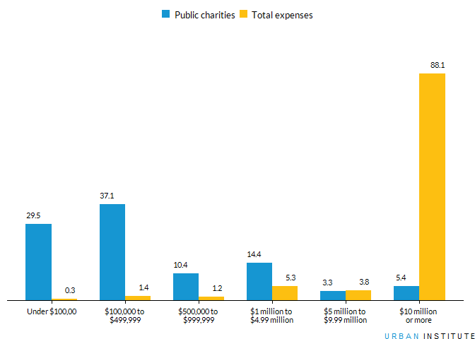
Even after excluding organizations with gross receipts below the $50,000 filing threshold, small organizations composed the majority of public charities in 2016. As shown in figure 1 below, 66.6 percent had less than $500,000 in expenses (211,782 organizations); they composed less than 2 percent of total public charity expenditures ($32.8 billion). Though organizations with $10 million or more included just 5.4 percent of total public charities (17,063 organizations), they accounted for 88.1 percent of public charity expenditures ($1.7 trillion).

FIGURE 1

_{Number and Expenses of Reporting Public Charities as a Percentage of All Reporting Public Charities and Expenses}

#Create and Display Figure For 2016 Data 
Fig1Plot <- function(expstable) {
 
  #select relevant fields
  expstable <- expstable[,c("year_of_data", "EXPCAT", "Public charities", "Total expenses")]
 
  #plot graph
  Fig1<- expstable %>%  
    #shift from wide to long
    melt() %>% 
    #create graph
    ggplot(aes(EXPCAT, value, fill=variable))+
    geom_bar(stat="identity", position="dodge") +
    geom_text(aes(EXPCAT, value, label=formatC(round(value,1), format = 'f', digits =1)),
              vjust=-1, 
              position = position_dodge(width=1),
              size =3) +
    #labs(
      #title = "Figure 1",
      #subtitle =  paste("Number and Expenses of Reporting Public Charities as a Percentage of All Reporting Public Charities and Expenses, ", expstable$year_of_data[1], sep =""),
      #caption = paste("Urban Institute, National Center for Charitable Statistics, Core Files (Public Charities, "
                         #, expstable$year_of_data[1], ")", sep ="")) +
    theme(axis.title.y = element_blank(),
          axis.text.y = element_blank(),
          axis.ticks.y = element_blank(),
          axis.title.x = element_blank(),
          panel.grid = element_blank()) +
    scale_y_continuous(expand = c(0, 0), limits = c(0,105)) +
    scale_x_discrete(labels = c("Under $100,00", "$100,000 to $499,999", "$500,000 to $999,999", "$1 million to $4.99 million",
                               "$5 million to $9.99 million", "$10 million or more")) 
 
 
  UrbCaption <- grobTree(
    gp = gpar(fontsize = 8, hjust = 1), 
    textGrob(label = "I N S T I T U T E", 
             name = "caption1",
             x = unit(1, "npc"),  
             y = unit(0, "npc"),
             hjust = 1, 
             vjust = 0),
    textGrob(label = "U R B A N  ", 
             x = unit(1, "npc") - grobWidth("caption1") - unit(0.01, "lines"),         
             y = unit(0, "npc"), 
             hjust = 1, 
             vjust = 0, 
             gp = gpar(col = "#1696d2")))
 
 
  grid.arrange(Fig1, UrbCaption, ncol = 1, heights = c(30, 1))
 
 
}
 
Fig1Plot(Figure1_2016)

Source: Urban Institute, National Center for Charitable Statistics, Core Files (Public Charities, 2016)

Type

#Create Table 2 Function
Table2 <- function(datayear) {
  #select core file based on year
  file <-  c(paste("core", datayear, "pc", sep =""))
 
  #get core file
  dataset <- get(file)
 
  #filter out organizations below minimum filing threshold for 990-EZ
  dataset <- if(datayear < 2010) filter(dataset, ((GRREC >= 25000)|(TOTREV>25000))) else filter(dataset, ((GRREC >= 50000)|(TOTREV>50000)))
 
  #create table
  Table2<- dataset %>%
    filter((OUTNCCS != "OUT"), (FNDNCD != "02" & FNDNCD!= "03" & FNDNCD != "04")) %>%
    group_by(NTEEGRP) %>%
    summarize( 
      Number_of_Orgs = n(),
      Revenue = round((sum(TOTREV, na.rm =TRUE))/1000000000, digits =1),
      Expenses = round((sum(EXPS, na.rm =TRUE))/1000000000, digits =1),
      Assets = round((sum(ASS_EOY, na.rm =TRUE))/1000000000, digits=1)) %>%
    mutate(
      Revenue_PCT = round((Revenue/sum(Revenue)) *100, digits =1),
      Expenses_PCT = round((Expenses/sum(Expenses)) *100, digits =1),
      Assets_PCT = round((Assets/sum(Assets)) *100, digits =1),
      Numbers_PCT = round((Number_of_Orgs/sum(Number_of_Orgs)) *100, digits =1)
    )
 
  #reorder columns
  Table2 <- Table2[,c("NTEEGRP", "Number_of_Orgs","Numbers_PCT","Revenue","Expenses", "Assets", "Revenue_PCT", "Expenses_PCT","Assets_PCT")]
 
  #Add total row
  myNumCols <- which(unlist(lapply(Table2, is.numeric)))
  Table2[(nrow(Table2) + 1), myNumCols] <- colSums(Table2[, myNumCols], na.rm=TRUE)
  Table2$NTEEGRP[11] = "All public charities"
 
  #add All Ed and All health rows
  Table2[12,1] = "Education"
  Table2[12,2:9] <- Table2[3,2:9] + Table2[7,2:9]
  Table2[13,1] = "Health"
  Table2[13,2:9] <- Table2[4,2:9] + Table2[8,2:9]
 
  #reorder table with new rows
  t2order <- c("All public charities", "Arts", "Education", "Higher education", "Other education", "Environment and animals",
               "Health", "Hospitals and primary care facilities", "Other health care", "Human services",
               "International", "Other public and social benefit", "Religion related")
 
  Table2 <- Table2 %>%
    slice(match(t2order, NTEEGRP))
 
  #add year of data column
  Table2 <- cbind(year_of_data = as.character(datayear), Table2)
 
  return(Table2)
 
}
 
#Run for Table 2 for 2015 data
Table2_2016 <- Table2(params$NCCSDataYr)
write.csv(Table2_2016, "Tables/NSiB_Table2.csv")

Table 2 below displays the 2016 distribution of public charities by type of organization. Human services groups—such as food banks, homeless shelters, youth services, sports organizations, and family or legal services—composed over one-third of all public charities (35.2 percent). They were more than twice as numerous as education organizations, the next-most prolific type of organization, which accounted for 17.2 percent of all public charities. Education organizations include booster clubs, parent-teacher associations, and financial aid groups, as well as academic institutions, schools, and universities. Health care organizations, though accounting for only 12.2 percent of reporting public charities, accounted for nearly three-fifths of public charity revenues and expenses in 2016. Education organizations accounted for 17.3 percent of revenues and 16.9 percent of expenses; human services, despite being more numerous, accounted for comparatively less revenue (11.9 percent of the total) and expenses (12.1 percent of the total). Hospitals, despite representing only 2.2 percent of total public charities (7,054 organizations), accounted for about half of all public charity revenues and expenses (49.8 and 50.6 percent, respectively).

TABLE 2

_{Number and Finances of Reporting Public Charities by Subsector, 2016}

#Display Table 2
kable(Table2_2016[c(2:10)], format.args = list(decimal.mark = '.', big.mark = ","), 
     "html",
      align = "lcccccccc",
      col.names = c("", "Number", "% of total", "Revenues", "Expenses", "Assets", "Revenues", "Expenses", "Assets")) %>%
  kable_styling("hover", full_width = F) %>%
  row_spec(c(4,5,8,9), italic = T ) %>%
  row_spec(1, bold = T ) %>%
  add_indent(c(4,5,8,9)) %>%
  add_header_above(c(" " = 3, "Dollar Total ($ billions)" = 3, "Percentage of Total" = 3)) 

			Dollar Total ($ billions)			Percentage of Total
	Number	% of total	Revenues	Expenses	Assets	Revenues	Expenses	Assets
All public charities	318,015	100.1	2,041.5	1,937.3	3,793.7	100.0	100.0	100.0
Arts	31,894	10.0	40.2	36.9	132.9	2.0	1.9	3.5
Education	54,632	17.2	353.8	327.9	1,144.8	17.3	16.9	30.2
Higher education	2,161	0.7	226.4	213.4	740.6	11.1	11.0	19.5
Other education	52,471	16.5	127.4	114.5	404.2	6.2	5.9	10.7
Environment and animals	14,932	4.7	19.8	17.2	50.8	1.0	0.9	1.3
Health	38,853	12.2	1,208.5	1,167.8	1,643.1	59.2	60.3	43.3
Hospitals and primary care facilities	7,054	2.2	1,016.0	980.1	1,339.1	49.8	50.6	35.3
Other health care	31,799	10.0	192.5	187.7	304.0	9.4	9.7	8.0
Human services	111,797	35.2	243.0	234.5	371.4	11.9	12.1	9.8
International	6,956	2.2	39.7	35.9	44.6	1.9	1.9	1.2
Other public and social benefit	38,071	12.0	117.1	99.3	369.0	5.7	5.1	9.7
Religion related	20,880	6.6	19.4	17.8	37.1	1.0	0.9	1.0

Source: Urban Institute, National Center for Charitable Statistics, Core Files (Public Charities, 2016).

Note: Subtotals may not sum to totals because of rounding.

Growth

#Create Table 3 function
Table3 <- function(datayear) {
 
  #define years of interest
  T3grab = function(yr) {
    output <- c(paste("core", yr-10, "pc", sep = ""), 
                paste("core", yr-5, "pc", sep =""),
                paste("core", yr, "pc", sep =""))
    return(list(output))
  }
 
 
  #define financial summarizer
  T3Fin <- function(dataset, year) {
    df <- get(dataset)
 
    #filter out organizations below minimum filing threshold for 990-EZ
    df <- if(year < 2010) filter(df, ((GRREC >= 25000)|(TOTREV>25000))) else filter(df, ((GRREC >= 50000)|(TOTREV>50000)))
 
    output <- df %>%
      filter((OUTNCCS != "OUT"), (FNDNCD != "02" & FNDNCD!= "03" & FNDNCD != "04")) %>%
      group_by(NTEEGRP) %>%
      summarize( 
        Number_of_Orgs = n(),
        Revenue = round((sum(as.numeric(TOTREV), na.rm =TRUE)/1000000000), digits =1),
        Expenses = round((sum(as.numeric(EXPS), na.rm =TRUE)/1000000000), digits=1),
        Assets = round((sum(as.numeric(ASS_EOY), na.rm =TRUE)/1000000000), digits=1)
) %>%
      mutate(
        Revenue = round((Revenue * inflindex[as.character(datayear),])/(inflindex[as.character(year),]), digits =1),
                Expenses = round((Expenses * inflindex[as.character(datayear),])/(inflindex[as.character(year),]), digits =1),
        Assets = round((Assets * inflindex[as.character(datayear),])/(inflindex[as.character(year),]), digits =1)
      )  
    colnames(output)[2:5] <- paste(colnames(output)[2:5], year, sep = "_")
    return(output)
  }
 
  #run grabber for years of interest
  T3years <-T3grab(datayear)
 
  #pull each year
  comp1 <- T3Fin(T3years[[1]][1], (datayear-10))
  comp2 <- T3Fin(T3years[[1]][2], (datayear-5))
  comp3 <- T3Fin(T3years[[1]][3], datayear)
 
  #merge tables
  Table3 <- comp1 %>%
    left_join(comp2, by = "NTEEGRP") %>%
    left_join(comp3, by = "NTEEGRP")
 
  #reorder columns
  Table3IA <- Table3[, c(1,2,6,10,3,7,11,4,8,12,5,9,13)]
 
  #Add total row
  myNumCols <- which(unlist(lapply(Table3IA, is.numeric)))
  Table3IA[(nrow(Table3IA) + 1), myNumCols] <- colSums(Table3IA[, myNumCols], na.rm=TRUE)
  Table3IA$NTEEGRP[11] = "All public charities"
 
  #add All Ed and All health rows
  Table3IA[12,1] = "Education"
  Table3IA[12,2:13] <- Table3IA[3,2:13] + Table3IA[7,2:13]
  Table3IA[13,1] = "Health"
  Table3IA[13,2:13] <- Table3IA[4,2:13] + Table3IA[8,2:13]
 
  #reorder table with new rows
  t3order <- c("All public charities", "Arts", "Education", "Higher education", "Other education", "Environment and animals",
               "Health", "Hospitals and primary care facilities", "Other health care", "Human services",
               "International", "Other public and social benefit", "Religion related")
 
  Table3IA <- Table3IA %>%
    slice(match(t3order, NTEEGRP))
 
  #add year of data column
  Table3IA <- cbind(year_of_data = as.character(datayear), Table3IA)
 
  return(Table3IA)
}
 
#Run Table 3 for 2016 data
Table3_2016 <- Table3(params$NCCSDataYr)
write.csv(Table3_2016, "Tables/NSiB_Table3.csv")
 
####################################################
 
#Create Table 4 function
Table4 <- function(datayear) {
 
  #start with table 3 data
  Table4 <- Table3(datayear)
 
  #calculate percentage change fields
  Table4 <- Table4 %>%
    mutate(
      RevAtoC = round(((Table4[,8] - Table4[,6] )/(Table4[,6] )) *100,1),
      RevAtoB = round(((Table4[,7]-  Table4[,6] )/(Table4[,6] )) *100,1),
      RevBtoC = round(((Table4[,8]-  Table4[,7] )/(Table4[,7] )) *100,1),
      ExpsAtoC =round(((Table4[,11] - Table4[,9] )/(Table4[,9] )) *100,1),
      ExpsAtoB =round(((Table4[,10]-  Table4[,9] )/(Table4[,9] )) *100,1),
      ExpsBtoC =round(((Table4[,11]-  Table4[,10] )/(Table4[,10] )) *100,1),
      AssAtoC = round(((Table4[,14] -Table4[,12] )/(Table4[,12] )) *100,1),
      AssAtoB = round(((Table4[,13]- Table4[,12] )/(Table4[,12] )) *100,1),
      AssBtoC = round(((Table4[,14]- Table4[,13])/(Table4[,13] ))*100,1)
 
    )
 
  #drop intermediary raw number columns
  Table4 <- Table4[-(3:14)]
 
  #rename columns by year
  colnames(Table4)[3] <- paste("Revenue", datayear-10, "\u2013", datayear, sep = "_")
  colnames(Table4)[4] <- paste("Revenue", datayear-10, "\u2013", datayear-5, sep = "_")
  colnames(Table4)[5] <- paste("Revenue", datayear-5, "\u2013", datayear, sep = "_")
  colnames(Table4)[6] <- paste("Expenses", datayear-10, "\u2013", datayear, sep = "_")
  colnames(Table4)[7] <- paste("Expenses", datayear-10, "\u2013", datayear-5, sep = "_")
  colnames(Table4)[8] <- paste("Expenses", datayear-5, "\u2013", datayear, sep = "_")
  colnames(Table4)[9] <- paste("Assets", datayear-10, "\u2013", datayear, sep = "_")
  colnames(Table4)[10] <- paste("Assets", datayear-10, "\u2013", datayear-5, sep = "_")
  colnames(Table4)[11] <- paste("Assets", datayear-5, "\u2013", datayear, sep = "_")
 
  #return output
  return(Table4)
 
}
 
#Run Table 4 for 2016 data
Table4_2016 <- Table4(params$NCCSDataYr)
write.csv(Table4_2016,"Tables/NSiB_Table4.csv")

The number of reporting public charities in 2016 was approximately 1 percent higher than the number in 2015. The total revenues, expenses, and assets for reporting public charities all increased between 2015 and 2016; after adjusting for inflation, revenues rose 1.9 percent, expenses rose 4 percent, and assets rose 2.1 percent.

These trends are indicative of larger growth in the sector: both the number and finances of organizations in the nonprofit sector have grown over the past 10 years. But this growth has differed by subsector and period (table 3). Subsectors experienced varying degrees of financial expansion: although all subsectors reported increases in revenue in 2016 compared with 2006 (even after adjusting for inflation), a few decreased in number of nonprofits, including arts, education (excluding higher education), health, and other public and social benefit organizations. Consequently, these organizations accounted for a slightly lower proportion of the total sector in 2016 (50.7 percent) than they did in 2006 (53.5 percent). The smallest subsectors (international and foreign affairs organizations and environment and animals organizations) saw the largest growth rates in the number of organizations, increasing 16 and 10.1 percent, respectively, from 2006 to 2016.

Financially, religion-related organizations had the largest proportional increase in both revenue and expenses, growing from $13.2 billion in revenue in 2006 to $19.4 billion in 2016 after adjusting for inflation (a change of 47 percent). Environment and animals organizations experienced similar growth, growing from $14.6 billion in revenue in 2006 to $19.8 billion in 2016 after adjusting for inflation (a change of 35.6 percent). Both types of organizations, however, still account for a very small proportion of overall nonprofit sector revenue in 2016, at just about 1 percent each. Health-related organizations, which account for a much larger proportion of overall sector finances (59.2, 60.3 and 43.3 percent, respectively, of revenues, expenses, and assets), also experienced considerable growth between 2006 and 2016. Revenues for hospitals and primary care facilities, in particular, increased from $739.7 billion in 2006 to $1016 billion in 2016 after adjusting for inflation, by far the largest dollar growth of any subsector during this period. The growth for the health sector, $331.4 billion, accounts for over three-fifths of the growth of the entire nonprofit sector between 2006 and 2016 ($505.1 billion).

TABLE 3

_{Number, Revenues, and Assets of Reporting Public Charities by Subsector, 2006–2016 (adjusted for inflation)}

#Display Table 3
kable(Table3_2016[c(2:14)], format.args = list(decimal.mark = '.', big.mark = ","), 
      "html",
      col.names = c("", "2006", "2011", "2016", "2006", "2011", "2016", "2006", "2011", "2016", "2006", "2011", "2016"),
      align = "lcccccccccccc"#,
          )%>%
  kable_styling("hover", full_width = F) %>%
  row_spec(c(4,5,8,9), italic = T ) %>%
  row_spec(1, bold = T ) %>%
  add_indent(c(4,5,8,9)) %>%
  add_header_above(c(" ", "Number of Organizations" = 3, "Revenue ($ billions)" = 3, "Expenses ($ billions)" = 3, "Assets ($ billions)" = 3)) 

	Number of Organizations			Revenue ($ billions)			Expenses ($ billions)			Assets ($ billions)
	2006	2011	2016	2006	2011	2016	2006	2011	2016	2006	2011	2016
All public charities	326,246	287,318	318,015	1,536.4	1,698.5	2,041.5	1,394.5	1,596.7	1,937.3	2,705.2	3,015.7	3,793.7
Arts	36,065	28,579	31,894	35.4	32.5	40.2	29.0	29.8	36.9	106.1	107.6	132.9
Education	58,663	49,223	54,632	273.7	286.8	353.8	225.1	259.8	327.9	835.8	906.8	1,144.8
Higher education	1,933	2,013	2,161	179.1	186.5	226.4	147.7	169.4	213.4	557.2	585.6	740.6
Other education	56,730	47,210	52,471	94.6	100.3	127.4	77.4	90.4	114.5	278.6	321.2	404.2
Environment and animals	13,565	12,547	14,932	14.6	15.8	19.8	11.9	14.2	17.2	34.9	38.2	50.8
Health	41,753	37,828	38,853	877.1	1,008.0	1,208.5	826.7	957.8	1,167.8	1,083.6	1,284.3	1,643.1
Hospitals and primary care facilities	7,266	7,093	7,054	739.7	854.5	1,016.0	702.3	811.7	980.1	858.6	1,040.1	1,339.1
Other health care	34,487	30,735	31,799	137.4	153.5	192.5	124.4	146.1	187.7	225.0	244.2	304.0
Human services	110,226	102,321	111,797	198.3	215.4	243.0	187.3	208.4	234.5	291.3	322.3	371.4
International	5,999	6,047	6,956	31.0	30.8	39.7	28.1	30.0	35.9	31.7	31.9	44.6
Other public and social benefit	40,029	33,365	38,071	93.1	94.7	117.1	74.9	83.5	99.3	292.5	292.7	369.0
Religion related	19,946	17,408	20,880	13.2	14.5	19.4	11.5	13.2	17.8	29.3	31.9	37.1

Source: Urban Institute, National Center for Charitable Statistics, Core Files (Public Charities, 2006, 2011, and 2016).

Note: Subtotals may not sum to totals because of rounding.

Public charities' financial growth within the given span largely occurred within the second half (table 4). From 2006 to 2011, revenue and assets for all public charities increased 10.6 and 11.5 percent, respectively, but both grew much more quickly in the years following: 20.2 percent for revenues and 25.8 percent for assets, after adjusting for inflation. Further, expenses grew much faster than revenues between 2006 and 2011, with expenses increasing 14.5 percent (compared with revenues increasing 10.6 percent). But between 2011 and 2016 growth in expenses (21.3 percent) was outpaced by the growth in revenues (20.2 percent).

These periods of growth varied by subsector, however. Two subsectors experienced declining revenue between 2006 and 2011: arts, culture, and humanities organizations and other public and social benefit organizations. Of the two, other public and social benefit organizations experienced the larger decline, falling $-1.6 billion in revenue from 2006 to 2011, a decline of -1.7 percent. However, both subsectors experienced substantial revenue increases from 2011 to 2016: revenue for other public and social benefit organizations grew 23.7 percent during those five years, while revenue for arts, culture and humanities organizations grew 23.7 percent. Both revenue growth rates were well above the growth rate for human services organizations, which at 12.8 percent was the lowest for any subsector within that period.

TABLE 4

_{Percent Change in Revenue, Expenses, and Assets of Reporting Public Charities by Subsector, 2006–2016 (adjusted for inflation)}

#Display Table 4 Data
kable(Table4_2016[c(2:11)], format.args = list(decimal.mark = '.', big.mark = ","), 
      "html",
      col.names = c("", paste("2006", "\u2014", "16", sep = ""), paste("2006", "\u2014", "11", sep = ""), paste("2011", "\u2014", "16", sep = ""), paste("2006", "\u2014", "16", sep = ""), paste("2006", "\u2014", "11", sep = ""), paste("2011", "\u2014", "16", sep = ""), paste("2006", "\u2014", "16", sep = ""), paste("2006", "\u2014", "11", sep = ""), paste("2011", "\u2014", "16", sep = "")),
      align = "lccccccccc") %>%
  kable_styling("hover", full_width = F) %>%
  row_spec(c(4,5,8,9), italic = T ) %>%
  row_spec(1, bold = T ) %>%
  add_indent(c(4,5,8,9)) %>%
  add_header_above(c(" ", "Change in Revenues" = 3, "Change in Expenses" = 3,"Change in Assets" = 3))

	Change in Revenues			Change in Expenses			Change in Assets
	2006—16	2006—11	2011—16	2006—16	2006—11	2011—16	2006—16	2006—11	2011—16
All public charities	32.9	10.6	20.2	38.9	14.5	21.3	40.2	11.5	25.8
Arts	13.6	-8.2	23.7	27.2	2.8	23.8	25.3	1.4	23.5
Education	29.3	4.8	23.4	45.7	15.4	26.2	37.0	8.5	26.2
Higher education	26.4	4.1	21.4	44.5	14.7	26.0	32.9	5.1	26.5
Other education	34.7	6.0	27.0	47.9	16.8	26.7	45.1	15.3	25.8
Environment and animals	35.6	8.2	25.3	44.5	19.3	21.1	45.6	9.5	33.0
Health	37.8	14.9	19.9	41.3	15.9	21.9	51.6	18.5	27.9
Hospitals and primary care facilities	37.4	15.5	18.9	39.6	15.6	20.7	56.0	21.1	28.7
Other health care	40.1	11.7	25.4	50.9	17.4	28.5	35.1	8.5	24.5
Human services	22.5	8.6	12.8	25.2	11.3	12.5	27.5	10.6	15.2
International	28.1	-0.6	28.9	27.8	6.8	19.7	40.7	0.6	39.8
Other public and social benefit	25.8	1.7	23.7	32.6	11.5	18.9	26.2	0.1	26.1
Religion related	47.0	9.8	33.8	54.8	14.8	34.8	26.6	8.9	16.3

Source: Urban Institute, National Center for Charitable Statistics, Core Files (Public Charities, 2006, 2011, and 2016).

Note: Subtotals may not sum to totals because of rounding.

Giving

Giving Amounts

#Create Figure 2 underlying table
 
#Import Figure 2 raw data (available from Giving USA 2018, https://givingusa.org/)
Figure2 <- read_csv("External_Data/GivingUSACont.csv",
                          col_types = cols_only(Years = col_integer(),
                                                Current_Dollars = col_double()
                                                                          ))
#Adjust for inflation
Figure2 <- Figure2 %>%
  mutate(
    'Constant (2017) Dollars' = round((Current_Dollars * inflindex[as.character(2018),])/(inflindex[as.character(Years),]), digits =2)
  )
#Add Column Names
colnames(Figure2)<- c("Year", "Current dollars", "Constant (2018) dollars")
 
Figure2 <- Figure2 %>%
  melt(id = "Year")
 
colnames(Figure2)[2] <- "Contributions"
 
#Write final table to CSV
write.csv(Figure2, "Figures/NSiB_Figure2_Table.csv")

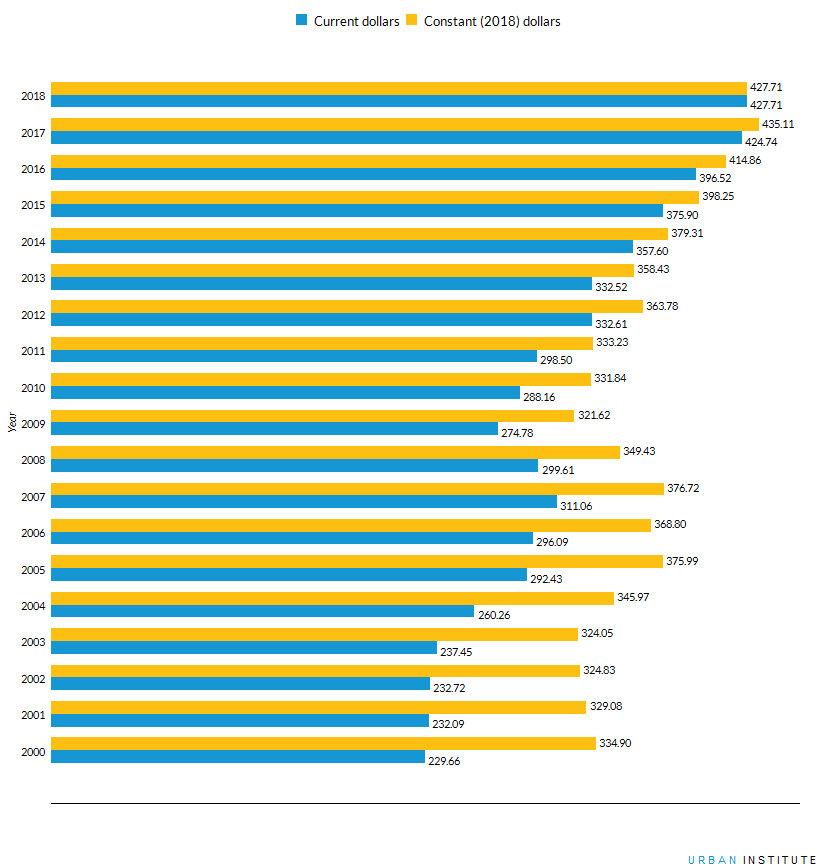
Private charitable contributions reached an estimated $427.71 billion in 2018, as shown in figure 2 below (Giving USA Foundation 2019). Although total charitable giving has been increasing for four consecutive years, beginning with 2014. In 2018, total charitable giving decreased -1.7 percent from 2017.

FIGURE 2

_{Private Charitable Contributions 2000-2018}

#Create Figure 2
Fig2Plot <- function(Fig2Table) {
 
  Fig2 <- Fig2Table %>%
    ggplot(aes(x=Year, y =value, fill = Contributions)) +
    geom_bar(position = "dodge", stat = "identity") +
    geom_text(aes(label = formatC(round(value,2), format = 'f', digits =2)),
              position= position_dodge(width=1), 
              hjust =-.1,
              size=3) +
    scale_y_continuous(expand = c(0, 0), limits = c(0,460)) +
    scale_x_continuous(breaks = 2000:2018)+
    theme(axis.text.x = element_blank(),
          axis.ticks.x = element_blank(),
          panel.grid.major = element_blank()#,
         # axis.title.y = element_text(angle=0)
          ) +
    labs(#title = "Figure 2",
         #subtitle = "Private Charitable Contributions, 2000-2016",
         #caption = "Giving USA Foundation (2018)",
         x = "Year",
         y = "") +
    coord_flip()
 
  UrbCaption <- grobTree(
    gp = gpar(fontsize = 8, hjust = 1), 
    textGrob(label = "I N S T I T U T E", 
             name = "caption1",
             x = unit(1, "npc"),  
             y = unit(0, "npc"),
             hjust = 1, 
             vjust = 0),
    textGrob(label = "U R B A N  ", 
             x = unit(1, "npc") - grobWidth("caption1") - unit(0.01, "lines"),         
             y = unit(0, "npc"), 
             hjust = 1, 
             vjust = 0, 
             gp = gpar(col = "#1696d2")))
 
 
  grid.arrange(Fig2, UrbCaption, ncol = 1, heights = c(30, 1))
}
 
Fig2Plot(Figure2)

Source: Giving USA Foundation (2019).

Recipients

#Create Table 5
 
#Import raw Table 5 data (available from Giving USA 2018, https://givingusa.org/)
Table5 <- read_csv("External_Data/GivingUSAType.csv",
                   col_types= cols_only(Type = col_character(),
                                        Year2013 = col_double(),
                                        Year2018 = col_double()))
#Calculate percentage change
Table5 <- Table5 %>%
  mutate(PCt_change = Year2018 - Year2013)
 
#Rename Columns
colnames(Table5)<- c("Charity type", "% of all contributions, 2013", "% of all contributions, 2018", paste("% point change, 2013", "\u2013", "18", sep =""))
 
#Write final table to CSV
write.csv(Table5, "Tables/NSiB_Table5.csv")

Congregations and religious organizations received just under a third (29.6 percent) of all charitable contributions in 2018 (table 5), a lower proportion than they received five years earlier in 2013 (32.2 percent). Education organizations received the next-highest share of private charitable contributions (13.9 percent), which is the same proportion received in 2013 (also 13 percent of all donations). Human services organizations received the third-highest pro portion of all contributions in 2018 (12.2 percent), but this is a slight decline from their 2013 proportion (12 percent). Gifts to individuals made up the smallest proportion of total contributions in 2018: 2.1 percent.

TABLE 5

_{Charitable Contributions by Type of Recipient Organizations, 2018}

#Display Table 5
kable(Table5, format.args = list(decimal.mark = '.', big.mark = ","), 
      "html",
      align = "lccc") %>%
  kable_styling("hover", full_width = F) 

Charity type	% of all contributions, 2013	% of all contributions, 2018	% point change, 2013–18
Religion	32.2	29.6	-2.6
Education	13.0	13.9	0.9
Human services	12.0	12.2	0.2
Gifts to foundations	11.9	11.9	0.0
Health	9.4	9.7	0.3
International affairs	5.7	5.4	-0.3
Public-society benefit	7.1	7.4	0.3
Arts, culture, and humanities	4.3	4.6	0.3
Environment and animals	2.5	3.0	0.5
Gifts to individuals	2.1	2.2	0.1

Source: Giving USA Foundation (2019).

Foundations

#Import Raw Figure 3 data (available from the Foundation Center Foundation Stats, http://data.foundationcenter.org/)
Figure3 <- read_csv("External_Data/FoundationCenter.csv",
                    col_types = cols_only(Year = col_integer(),
                                          Foundations = col_integer(),
                                          Grants = col_double(),
                                          Assets = col_double()
                    ))
#Adjust for inflation
Figure3 <- Figure3 %>%
  mutate(
    Constant_Grants = round((Grants * inflindex[as.character(2017),])/(inflindex[as.character(Year),]), digits =1),
    Constant_Assets = round((Assets * inflindex[as.character(2017),])/(inflindex[as.character(Year),]), digits =1) 
  )
 
#write final table to csv
write.csv(Figure3, "Figures/NSiB_Figure3_Table.csv")

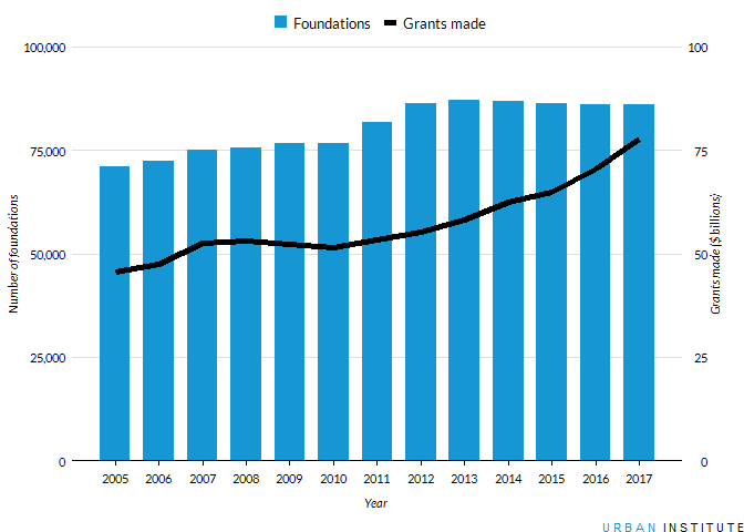
The Foundation Center (2019) estimates there were more than 86,125 grantmaking foundations in the United States in 2017. Their grants, a component of private charitable contributions, totaled $77.7 billion in 2017, up 10.4 percent from 2016 after adjusting for inflation (figure 3). Between 2005 and 2017, foundation grantmaking increased 70 percent after adjusting for inflation. Foundation assets also grew over the same period, increasing 46.6 percent from $691 billion in 2005 to $1012.9 billion in 2017 after adjusting for inflation.

FIGURE 3

_{Number of Foundations and Amount of Grants Made by Year, 2005-2017}

#Graph Figure 3 Table
Fig3Plot <- function(Fig3Table) {
 
  Fig3 <- Fig3Table %>%
    ggplot(aes(x=Year)) +
    geom_bar(aes(y=Foundations, fill= "Foundations"), stat = "identity") +
    geom_line(aes(y=Constant_Grants*1000, color = "Grants made"), size = 2) +
    scale_y_continuous(expand = c(0, 0), limits = c(0,100000),
                       sec.axis = sec_axis(~./1000, name = "Grants made ($ billions)"),
                       labels = scales::comma) +
    scale_x_continuous(breaks = 2005:2017)+
    labs(#caption = "The Foundation Center, Foundation Stats (2019)",
         x = "Year",
         y = "Number of foundations") +
    scale_color_manual("", values = c("Foundations" = "#1696d2", "Grants made" = "black")) +
    scale_fill_manual("  ", values = "#1696d2")
 
  UrbCaption <- grobTree(
    gp = gpar(fontsize = 8, hjust = 1), 
    textGrob(label = "I N S T I T U T E", 
             name = "caption1",
             x = unit(1, "npc"),  
             y = unit(0, "npc"),
             hjust = 1, 
             vjust = 0),
    textGrob(label = "U R B A N  ", 
             x = unit(1, "npc") - grobWidth("caption1") - unit(0.01, "lines"),         
             y = unit(0, "npc"), 
             hjust = 1, 
             vjust = 0, 
             gp = gpar(col = "#1696d2")))
 
  grid.arrange(Fig3, UrbCaption, ncol = 1, heights = c(30, 1))
}
 
Fig3Plot(Figure3)

Source: The Foundation Center, Foundation Stats (2019).

Volunteering

#Calculate proportion of volunteering hours
#Data taken from Bureau of Labor Statistics: American Time Use Survey 2018 (https://www.bls.gov/tus/datafiles_2018.htm)
 
#Data downloaded and saved locally, read in files:
respondent18 <- read_csv("External_Data/atusresp_2017.dat", na = "-1")
activity18 <- read_csv("External_Data/atussum_2017.dat", na = "-1")

#Code to analyze American Time Use Survey Data
 
#Step 1: change variable names to lowercase
names(respondent18) <- tolower(names(respondent18))
names(activity18) <- tolower(names(activity18))
 
#Step 2: join respondent and activity data
atus18 <- left_join(respondent18, activity18, by = "tucaseid")
 
#Step 3: Create volunteering subset by filtering cases without any volunteering hours
atus18vol <- atus18 %>%
  filter(t150101>0 | 
           t150102>0 | 
           t150103>0 | 
           t150104>0 | 
           t150105>0 | 
           t150106>0 | 
           t150199>0 | 
           t150201>0 | 
           t150202>0 | 
           t150203>0 | 
           t150204>0 | 
           t150299>0 | 
           t150301>0 | 
           t150302>0 | 
           t150399>0 | 
           t150401>0 | 
           t150402>0 | 
           t150499>0 | 
           t150501>0 | 
           t150599>0 | 
           t150601>0 | 
           t150602>0 | 
           t150699>0 | 
           t150701>0 | 
           t150799>0 | 
           #t150801>0 | #(note: commented out because not available in 2017 ATUS)
           #t150899>0 |  #(note: commented out because not available in 2017 ATUS)
           t159999>0 | 
           t181501>0 | 
           t181599>0)
 
#Step 4: calculate weighted volunteering hours
atus18vol <- atus18vol %>%
  mutate(
    t150101w = tufinlwgt.x* t150101,
    t150102w = tufinlwgt.x* t150102, 
    t150103w = tufinlwgt.x* t150103, 
    t150104w = tufinlwgt.x* t150104, 
    t150105w = tufinlwgt.x* t150105, 
    t150106w = tufinlwgt.x* t150106, 
    t150199w = tufinlwgt.x* t150199, 
    t150201w = tufinlwgt.x* t150201, 
    t150202w = tufinlwgt.x* t150202, 
    t150203w = tufinlwgt.x* t150203, 
    t150204w = tufinlwgt.x* t150204, 
    t150299w = tufinlwgt.x* t150299, 
    t150301w = tufinlwgt.x* t150301, 
    t150302w = tufinlwgt.x* t150302, 
    t150399w = tufinlwgt.x* t150399, 
    t150401w = tufinlwgt.x* t150401, 
    t150402w = tufinlwgt.x* t150402, 
    t150499w = tufinlwgt.x* t150499, 
    t150501w = tufinlwgt.x* t150501, 
    t150599w = tufinlwgt.x* t150599, 
    t150601w = tufinlwgt.x* t150601, 
    t150602w = tufinlwgt.x* t150602, 
    t150699w = tufinlwgt.x* t150699, 
    t150701w = tufinlwgt.x* t150701, 
    t150799w = tufinlwgt.x* t150799, 
    #t150801w = tufinlwgt.x* t150801, (note: commented out because not available in 2017 ATUS)
    #t150899w = tufinlwgt.x* t150899, (note: commented out because not available in 2017 ATUS)
    t159999w = tufinlwgt.x* t159999, 
    t181501w = tufinlwgt.x* t181501, 
    t181599w = tufinlwgt.x* t181599
  )
 
#Step 5: Create reduced file of only weighted data
atus18vol <- atus18vol %>%
  select(tucaseid, 
         t150101w,
         t150102w,
         t150103w,
         t150104w,
         t150105w,
         t150106w,
         t150199w,
         t150201w,
         t150202w,
         t150203w,
         t150204w,
         t150299w,
         t150301w,
         t150302w,
         t150399w,
         t150401w,
         t150402w,
         t150499w,
         t150501w,
         t150599w,
         t150601w,
         t150602w,
         t150699w,
         t150701w,
         t150799w,
         #t150801w, (note: commented out because not available in 2017 ATUS)
         #t150899w, (note: commented out because not available in 2017 ATUS)
         t159999w,
         t181501w,
         t181599w,
         tufinlwgt.x)
 
 
 
#Step 6: Create categorical groupings, number of volunteer hours
atus18vol <- atus18vol %>%
  mutate( 
    adminsupport = t150101w + t150102w + t150103w + t150104w + t150105w + t150106w +t150199w,
    socialservice = t150201w + t150202w + t150203w + t150204w + t150299w,
    maintenance = t150301w + t150302w+ t150399w,
    performculture = t150401w + t150402w + t150499w,
    attendmeet = t150501w + t150599w,
    pubhealth = t150601w + t150602w + t150699w,
    waiting = t150701w + t150799w,
    #security = t150801w,
    travel = t181501w + t181599w,
    othervol = t159999w
  )
 
#Step 7: Calculate proprotion of weighted individuals involved in each category
 
#Step 7a: Administrative/Support
atus18vol$adminsupportprop <- ifelse((atus18vol$t150101w + 
                                        atus18vol$t150102w + 
                                        atus18vol$t150103w + 
                                        atus18vol$t150104w +
                                        atus18vol$t150105w + 
                                        atus18vol$t150106w + 
                                        atus18vol$t150199w) >0, 
                                     atus18vol$tufinlwgt.x, 
                                     0)
 
#Step 7b: Social service
atus18vol$socialserviceprop <- ifelse((atus18vol$t150201w + 
                                         atus18vol$t150202w + 
                                         atus18vol$t150203w + 
                                         atus18vol$t150204w +
                                         atus18vol$t150299w) >0, 
                                      atus18vol$tufinlwgt.x, 
                                      0)
 
#Step 7c: Maintenance
atus18vol$maintenanceprop <- ifelse((atus18vol$t150301w + 
                                       atus18vol$t150302w +
                                       atus18vol$t150399w) >0, 
                                    atus18vol$tufinlwgt.x, 
                                    0)
 
#Step 7d: Perform culture
atus18vol$performcultureprop <- ifelse((atus18vol$t150401w + 
                                          atus18vol$t150402w +
                                          atus18vol$t150499w) >0, 
                                       atus18vol$tufinlwgt.x, 
                                       0)
 
#Step 7e: Attend meetings
atus18vol$attendmeetprop <- ifelse((atus18vol$t150501w+
                                      atus18vol$t150599w) >0, 
                                   atus18vol$tufinlwgt.x, 
                                   0)
 
#Step 7f: Public health
atus18vol$pubhealthprop <- ifelse((atus18vol$t150601w + 
                                     atus18vol$t150602w +
                                     atus18vol$t150699w) >0, 
                                  atus18vol$tufinlwgt.x, 
                                  0)
 
#Step 7g: Waiting
atus18vol$waitingprop <- ifelse((atus18vol$t150701w + 
                                   atus18vol$t150799w) >0, 
                                atus18vol$tufinlwgt.x, 
                                0)
 
#Step 7h: Security
#atus18vol$securityprop <- ifelse((atus18vol$t150801w) >0, 
                                 #atus18vol$tufinlwgt.x, 
                                 #0)
 
#Step 7i: Travel
atus18vol$travelprop <- ifelse((atus18vol$t181501w + 
                                  atus18vol$t181599w) >0, 
                               atus18vol$tufinlwgt.x, 
                               0)
 
#Step 7j: Other
atus18vol$othervolprop <- ifelse((atus18vol$t159999w) >0, 
                                 atus18vol$tufinlwgt.x, 
                                 0)
 
#Step 8: Summarize number of hours/volunteers in each category
atus18volsum<- atus18vol %>%
  summarise(
    adminsupportprop = sum(adminsupportprop),
    socialserviceprop = sum(socialserviceprop),
    maintenanceprop = sum(maintenanceprop),
    performcultureprop = sum(performcultureprop),
    attendmeetprop = sum(attendmeetprop),
    pubhealthprop = sum(pubhealthprop),
    waitingprop = sum(waitingprop),
    #securityprop = sum(securityprop),
    travelprop = sum(travelprop),
    othervolprop = sum(othervolprop),
    adminsupport = sum(adminsupport),
    socialservice = sum(socialservice),
    maintenance= sum(maintenance),
    performculture = sum(performculture),
    attendmeet = sum(attendmeet),
    pubhealth = sum(pubhealth),
    waiting = sum(waiting),
    #security = sum(security),
    travel = sum(travel),
    othervol = sum(othervol)
  ) 
 
#Step 9: Reduce to number of volunteer hours
atus18volhours<- atus18volsum %>%
  select(adminsupport, socialservice, maintenance,  performculture, attendmeet, pubhealth, waiting, 
         #security, 
         travel, othervol) %>%
  gather(adminsupport, socialservice, maintenance,  performculture, attendmeet, pubhealth, waiting, 
         #security, 
         travel, othervol,
         key = "type",
         value = "hours")
 
 
#Step 10: rename columns
atus18volhours$type[grepl("adminsupport",atus18volhours$type )] <- "Administrative and support"
atus18volhours$type[grepl("socialservice",atus18volhours$type )] <- "Social service and care"
atus18volhours$type[grepl("maintenance",atus18volhours$type )] <- "Maintenance, building, and cleanup"
atus18volhours$type[grepl("performculture",atus18volhours$type )] <- "Performing and cultural activities"
atus18volhours$type[grepl("attendmeet",atus18volhours$type )] <- "Meetings, conferences, and training"
atus18volhours$type[grepl("pubhealth",atus18volhours$type )] <- "Public health and safety"
atus18volhours$type[grepl("waiting",atus18volhours$type )] <- "Waiting"
#atus18volhours$type[grepl("security",atus18volhours$type )] <- "Security procedures"
atus18volhours$type[grepl("travel",atus18volhours$type )] <- "Travel"
atus18volhours$type[grepl("othervol",atus18volhours$type )] <- "Other"
atus18volhours$type[grepl("adminsupport",atus18volhours$type )] <- "Administrative and support"
 
#Step 11: Calculate total
atus18volhours[10,2] <-sum(atus18volhours$hours)
atus18volhours$type[10] = "Total"
 
#Step 12: Calculate proportional number of hours per category
atus18volhours <-atus18volhours %>%
  mutate(
    AsPct = round(((hours/hours[10])*100),1)
  )
 
#Step 12: Remane final underlying table and write to CSV
Figure4 <- atus18volhours
write.csv(Figure4, "Figures/NSiB_Figure4_Table.csv")

#Read in Table 6 raw data
#Based on US Department of Labor, Bureau of Labor Statistics, Current Population Survey, Volunteer Supplement (2007-2015) (https://www.bls.gov/cps/home.htm),
#US Department of Labor, Bureau of Labor Statistics, American Time Use Survey (2008-2017) (https://www.bls.gov/tus/home.htm), 
#US Department of Labor, Bureau of Labor Statistics, Current Employment Statistics (2017) (https://www.bls.gov/ces/), and
#US Census Bureau "Annual Estimates of the Resident Population by Sex, Age, Race, and Hispanic Origin for the United States and States: April 1,2010 to July 1, 2017", (https://factfinder.census.gov/)
 
#Read in raw data, and write to CSV
Table6 <- read_csv("External_Data/Volunteering Data.csv")
write.csv(Table6, "Tables/NSiB_Table6.csv")

Volunteering is an important component of the nonprofit sector: over two-fifths of public charities rely on volunteers. ⁵ In previous nonprofit sector briefs, volunteering estimates were based on data from the Current Population Survey (CPS). Volunteer statistics from the CPS Volunteer Supplement are not available after September 2015: current figures shown here for total hours volunteered and total number of volunteers are based on previous estimates. For ongoing volunteering data updates, please visit https://www.nationalservice.gov/serve/via ⁶

Number of Volunteers

An estimated 64.4 million adults, 25.1 percent of the population volunteered at least once in 2017. The highest volunteer rate reported in the decade spanning from 2008 to 2017 was 26.8 percent, which was reported in 2009 and 2011. The lowest volunteer rate was reported in 2015: 24.9 percent.

The percentage of the population volunteering on a given day increased slightly in 2017, rising to 6 percent from 5.6 percent in 2016. This rise occurs after 2016 saw the lowest proportion of the population volunteering on an average day within the previous 10 years: however, the 15.6 people volunteering on a given day represents an increase of over 1 million daily volunteers from 2016. In the past decade, the highest proportion of Americans volunteering on a given day was in 2009, when 7.1 percent of the population volunteered (17.1 people).

Hours Volunteered

Americans volunteered an estimated 64.4 hours in 2017, a slight increase from 63.9 hours in 2016. This amounts to about 8.8 hours per volunteer, slightly more than in 2016.

Volunteer Activities

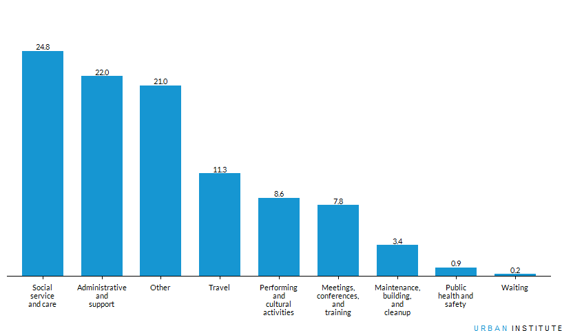
Figure 4 provides more information on how volunteers spent their time in 2018. The largest use of volunteer hours in 2018 was on social service and care activities (22 percent). These activities include such tasks as preparing food, collecting and delivering clothing or other goods, providing care, and teaching, counseling, or mentoring. Administrative and support activities made up the next-largest proportion of volunteer time (24.8 percent); this category includes things like computer use, telephone calls (except hotline counseling), writing, fundraising, and the like. These two categories of activities also led volunteer hours in 2017, although the proportion of time spent in social service and care activities has decreased slightly (from 24.8 percent) while the proportion of time spent in social administrative and support activities increased slightly (from 22 percent). Volunteers spent a larger proportion of their time in performing or cultural activities and meetings, conferenecs, and trainings in 2018 than in 2017, while they spent less time in maintenance, building, and cleanup activities.

FIGURE 4

_{Distribution of Volunteer Time by Acitivty, 2018 (percent)}

#Display Figure 4
Fig4Plot <- function(Fig4Table) {
 
  Fig4<- Fig4Table %>%
    filter(type != "Total") %>%
    #filter(type != "Security procedures") %>% #Filtered out because equals 0%
    ggplot(aes(x=reorder(type, -AsPct), y =AsPct)) +
    geom_bar(stat = "identity") +
    geom_text(aes(label=formatC(round(AsPct,1), format = 'f', digits =1)),
              position= position_dodge(width=1), 
              vjust =-.3,
              size=3) +
    scale_y_continuous(expand = c(0, 0), limits = c(0,30)) +
    labs(y = "Percent of total volunteer time") +
    theme(axis.title = element_blank(),
          panel.grid.major = element_blank(),
          axis.text.y = element_blank()) +
    scale_x_discrete(labels = function(type) str_wrap(type, width=10))
 
  UrbCaption <- grobTree(
    gp = gpar(fontsize = 8, hjust = 1), 
    textGrob(label = "I N S T I T U T E", 
             name = "caption1",
             x = unit(1, "npc"),  
             y = unit(0, "npc"),
             hjust = 1, 
             vjust = 0),
    textGrob(label = "U R B A N  ", 
             x = unit(1, "npc") - grobWidth("caption1") - unit(0.01, "lines"),         
             y = unit(0, "npc"), 
             hjust = 1, 
             vjust = 0, 
             gp = gpar(col = "#1696d2")))
 
  grid.arrange(Fig4, UrbCaption, ncol = 1, heights = c(30, 1))
}
 
Fig4Plot(Figure4)

Source: Author's calculations based on US Department of Labor, Bureau of Labor Statistics, American Time Use Survey 2018.

Value of Volunteering

The time volunteers spent in 2017 was worth an estimated 256 (table 6). The value of volunteer time combined with private giving accounted for over half a trillion dollars ($435.31 billion); volunteer time represents 12.9 percent of that total.

TABLE 6

_{Number, Hours, and Dollar Value of Volunteers, 2008-2017}

#Display Table 6
kable(Table6,  
      "html", 
      format.args = list(decimal.mark = '.', big.mark = ","),
      align = "lcccccccccc",
      col.names = c("", "2008", "2009", "2010", "2011", "2012", "2013", "2014", "2015", "2016", "2017")) %>%
  kable_styling("hover", full_width = F) %>%
  row_spec(c(1,7,11), bold = T, hline_after = T ) 

	2008	2009	2010	2011	2012	2013	2014	2015	2016	2017
Per year
Percent of population volunteering	26.4	26.8	26.3	26.8	26.5	25.4	25.3	24.9	25.2	25.1
Number of volunteers (millions)	61.8	63.4	62.8	64.3	64.5	62.6	62.8	62.6	63.9	64.4
Hours volunteered (billions)	8	8.1	8.1	8.5	8.5	8.3	8.7	8.5	8.7	8.8
Average hours per volunteer	130	128	129	132	132	133	139	136	136	137
Median hours per volunteer	52	52	52	51	50	50	50	52	--	--
Per average day
Percent of population volunteering	6.8	7.1	6.8	6	5.8	6.1	6.4	6.4	5.6	6
Number of volunteers (millions)	16.2	17.1	16.6	14.6	14.3	15.1	16	16.3	14.4	15.6
Hours per day per volunteer	2.43	2.39	2.46	2.84	2.48	2.57	2.41	2.49	2.39	2.86
Value of volunteers
Population age 16 and over (millions)	234.4	236.3	238.3	240	243.8	246.2	248.4	251.3	253.6	256
Full-time-equivalent employees (millions)	4.7	4.8	4.8	5	5	4.9	5.1	5	5.1	5.2
Assigned hourly wages for volunteers	$18.08	$18.63	$19.07	$19.47	$19.75	$20.16	$20.59	$21.08	$21.63	$22.13
Assigned value of volunteer time ($ billions)	$144.70	$150.70	$154.10	$164.80	$168.30	$167.20	$179.20	$179.00	$187.40	$195.00

Sources: Author's calculations based on data from US Department of Labor, Bureau of Labor Statistics, Current Population Survey, Volunteer Supplement (2007–16); US Department of Labor, Bureau of Labor Statistics, American Time Use Survey (2007–16); and US Department of Labor, Bureau of Labor Statistics, Current Employment Statistics (2016).

Notes: Median hours per volunteer not available for 2016 – 17. Percent of population volunteering and hours volunteered for 2016 – 17 estimated based on previous years.

Conclusion

Overall, in 2018, the nonprofit sector remained relatively healthy with continuous financial growth and increases in the number of nonprofits throughout various subsectors. However, new data in charitable giving trends point to nuances worthof further exploration. Public charities composed over two-thirds of all registered nonprofit organizations and accounted for over three-quarters of the revenue andexpenses of the nonprofit sector in the United States. From 2011 to 2016, the number of nonprofit organizations registered with the IRS rose by 4.5 percent. Nonprofit revenues grew 1.8 percent; assets increased 2.3 percent; and expenses grew by 3.6 percent.

While the nonprofit sector as a whole continues to see steady financial growth (with revenue, expenses, and assets all continuing to grow),” U.S. giving data points to new nuances in charitable giving worth disentangling. While annual levels of giving remained relatively steady since the Great Recession, pointing to an overall increase of 0.7 percent in giving between 2017 and 2018, after adjusting for inflation, private charitable giving shows a downward trend in total charitable giving. Disentangling this nuance will help better inform the overall state of nonprofit sector in the United States.

References

Foundation Center. 2018. Foundation Stats (2014). New York: Foundation Center. http://data.foundationcenter.org/#/foundations/all/nationwide/total/list/2014

Giving USA Foundation. 2018. Giving USA 2018: The Annual Report on Philanthropy for the Year 2017. Bloomington, IN: Giving USA Foundation.

Acknowledgments

*This brief was funded by the Urban Institute. The views expressed are those of the author and should not be attributed to the Urban Institute, its trustees, or its funders. Funders do not determine research findings or the insights and recommendations of Urban experts. Further information on the Urban Institute's funding principles is available at urban.org/fundingprinciples. *

Notes

GDP estimates are from the Bureau of Economic Analysis and include nonprofit institutions serving households. They exclude nonprofit institutions serving government or business. See table 1.3.5: Gross Value Added by Sector at “National Income and Product Accounts: National Data: Section 1 - Domestic Product and Income,” Bureau of Economic Analysis, accessed May 11, 2020, https://www.bea.gov/iTable/iTable.cfm?reqid=19&step=2#reqid=19&step=2&isuri=1&1921. ↩︎
The standard source for estimates of religious congregations is American Church lists, a company that provides marketing data using phone listings and other sources. The most recent estimates from American Church lists suggest that there are about 345,000 houses of worship in the United States. Of these, approximately 240,000 are registered with the IRS, according to National Center for Charitable Statistics's analysis of the February 2016 IRS Business Master File. See “Churches Mailing Lists and Sales Leads,” InfoUSA, accessed May 1, 2018, https://www.infousa.com/product/church-list/. ↩︎
All private foundations, regardless of size, are required to file a Form 990-PF. Before tax year 2010, nonprofits with gross receipts of $25,000 or more (excluding religious congregations) were required to file a Form 990 or Form 990-EZ. Beginning in 2010, only organizations with $50,000 or more in gross receipts (excluding religious congregations) are required to file a Form 990 or Form 990-EZ. Organizations with less than $50,000 in gross receipts are required to file an information return known as the Form 990-N (e-Postcard). Filing requirements by year are available at “Form 990 Series Which Forms Do Exempt Organizations File Filing Phase In,” Internal Revenue Service, accessed May 1, 2018, https://www.irs.gov/charities-non-profits/form-990-series-which-forms-do-exempt-organizations-file-filing-phase-in. ↩︎
Table 1 lists little change in the number of reporting charities between 2006 and 2016, with a growth rate of only -2.5 percent; it also lists the number of reporting charities falling 11.9 percent between 2006 and 2011. As noted in previous editions of “The Nonprofit Sector in Brief,” the 2012 National Center for Charitable Statistics Core File showed a substantial decrease from previous years. Because of IRS changes in data processing, we cannot conclusively verify the reason for this change. However, National Center for Charitable Statistics analysis suggests that this is likely caused by the introduction of new IRS filing guidelines and database management. With the introduction of the Form 990-N (e-Postcard), many smaller organizations were no longer required to file the full Form 990 or Form 990-EZ. Many organizations that had opted to file a Form 990 or Form 990-EZ (despite being under the minimum filing threshold) instead filed a Form 990-N for the 2012 tax period and afterward, and those Form 990-N filers are not counted as reporting organizations in table 1. The number of reporting charities increased 9.7 percent between 2011 and 2016—and, indeed, increased 2.3 percent between 2012 and 2013—suggesting that the sector continues to grow. Thus, the decline in number of reporting organizations between 2006 and 2011 reported here compared with editions of “The Nonprofit Sector in Brief” before 2014 should be understood as a reflection of the change in IRS filing guidelines. ↩︎
National Center for Charitable Statistics calculations of IRS Statistics of Income Division Exempt Organizations Sample (2012). ↩︎
Estimates of number of hours volunteered are based on data from the Current Population Survey (CPS). Volunteer statistics from the CPS Volunteer Supplement are not available after September 2015: 2016 figures for total hours volunteered and total number of volunteers are estimated from historical CPS data. Three years of data (2013–2015) were used to estimates 2016 volunteer rate and hours per capita. These rates were applied to Census Bureau estimates of the 16-and-over population (which includes people in the military or living in institutionalized housing) to project the sizes of the 2016 CPS 16-and-over population from the 2014 and 2015 estimates. For more on the CPS, see “Labor Force Statistics from the Current Population Survey,” Bureau of Labor Statistics, accessed May 1, 2018, https://www.bls.gov/cps/home.htm. For more on the American Time Use Survey, see “American Time Use Survey,” Bureau of Labor Statistics, accessed May 1, 2018, https://www.bls.gov/tus/home.htm. For more on the Census Bureau population estimates, see “Annual Estimates of the Resident Population by Sex, Age, Race, and Hispanic Origin for the United States and States: April 1,2010 to July 1, 2016,” US Census Bureau, available at American Fact Finder, accessed May 10, 2018, https://factfinder.census.gov/. ↩︎