This guide will teach you the concepts and code you will need for mapping and geospatial analysis in R. This is a long guide, so if you need something specific, we encourage you to scroll to the appropriate section using the Table of Contents on the left. If you just want copy and pasteable code to create different kinds of maps, head to the Map Gallery.
Now let’s start mapping!
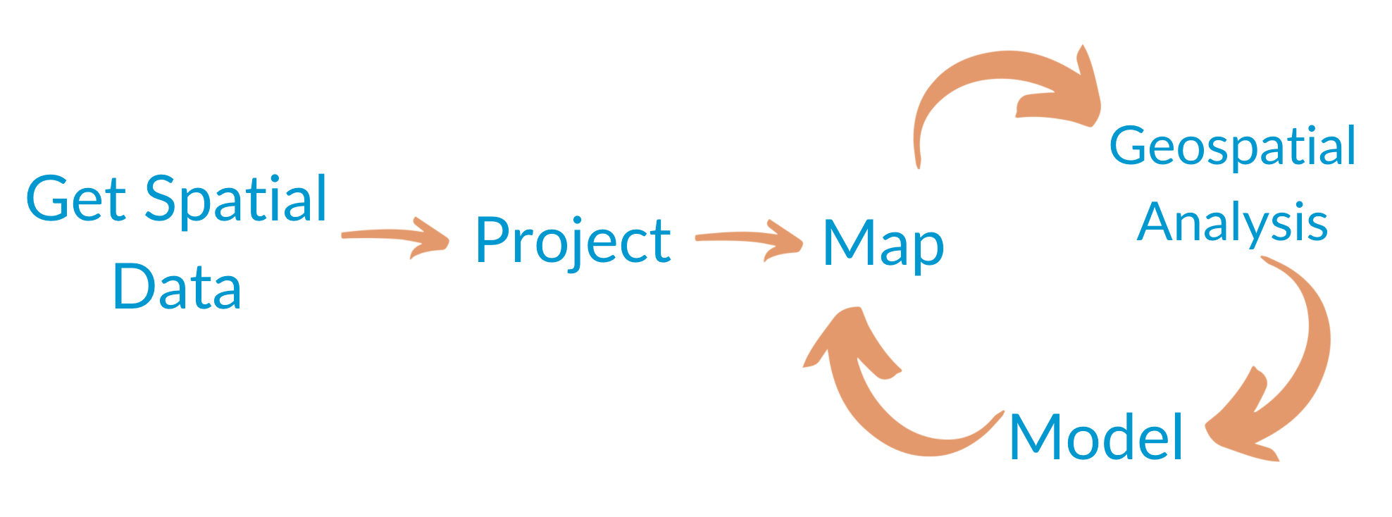
Geospatial Workflow
This picture below outlines what we think are the main steps in a geospatial workflow. This guide will be split into sections describing each of the steps.
Just because you’ve got geographic data, doesn’t mean that you have to make a map. Many times, there are more efficient storyforms that will get your point across more clearly. If your data shows a very clear geographic trend or if the absolute location of a place or event matters, maps might be the best approach, but sometimes the reflexive impulse to map the data can make you forget that showing the data in another form might answer other—and sometimes more important—questions.
So we would encourage you to think critically before making a map.
Why map with R?
R can have a steeper learning curve than point-and-click tools - like QGIS or ArcGIS - for geospatial analysis and mapping. But creating maps in R has many advantages including:
Reproducibility: By creating maps with R code, you can easily share the outputs and the code that generated the output with collaborators, allowing them to replicate your work and catch errors easily.
Iteration: With point and click software like ArcGIS, making 50 maps would be 50 times the work/time. But using R, we can easily make make many iterations of the same map with a few changes to the code.
Easy Updates: Writing code provides a roadmap for others (and future you!) to quickly update parts of the map as needed. Say for example a collaborator wanted to change the legend colors of 50 state maps. With R, this is possible in just a few seconds!
An Expansive ecosystem: There are several R packages that make it very easy to get spatial data, create static and interactive maps, and perform spatial analyses. This feature rich package ecosystem which all play nice together is frankly unmatched by other programming languages and even point and click tools like QGIS and ArcGIS. Some of these R packages include:
sf: For managing and analyzing spatial dataframes
tigris: For downloading in Census geographies
ggplot2: For making publication ready static maps
urbnmapr: For automatically adding Urban styling to static maps
mapview: For making expxploratory interactive maps
Cost: Most point-and-click tools for geospatial analysis are proprietary and expensive. R is free open-source software. The software and most of its packages can be used for free by anyone for almost any use case.
Helpful Learning Resources
In addition to this guide, you may want to look at these other helpful resources:
library(sf) stores geospatial data, which are points (a single longitude/latitude), lines (a pair of connected points), or polygons (a collection of points which make a polygon) in a geometry column within R dataframes
This is what sf dataframe looks like in the console:
dc_parks <-st_read("mapping/data/dc_parks.geojson", quiet =TRUE)# Print just the NAME and geometry columndc_parks %>%select(NAME) %>%head(2)
Simple feature collection with 2 features and 1 field
Geometry type: MULTIPOLYGON
Dimension: XY
Bounding box: xmin: -77.01063 ymin: 38.81718 xmax: -76.9625 ymax: 38.89723
Geodetic CRS: WGS 84
NAME geometry
1 Kingman and Heritage Islands MULTIPOLYGON (((-76.96566 3...
2 Bald Eagle Hill MULTIPOLYGON (((-77.01063 3...
The long version
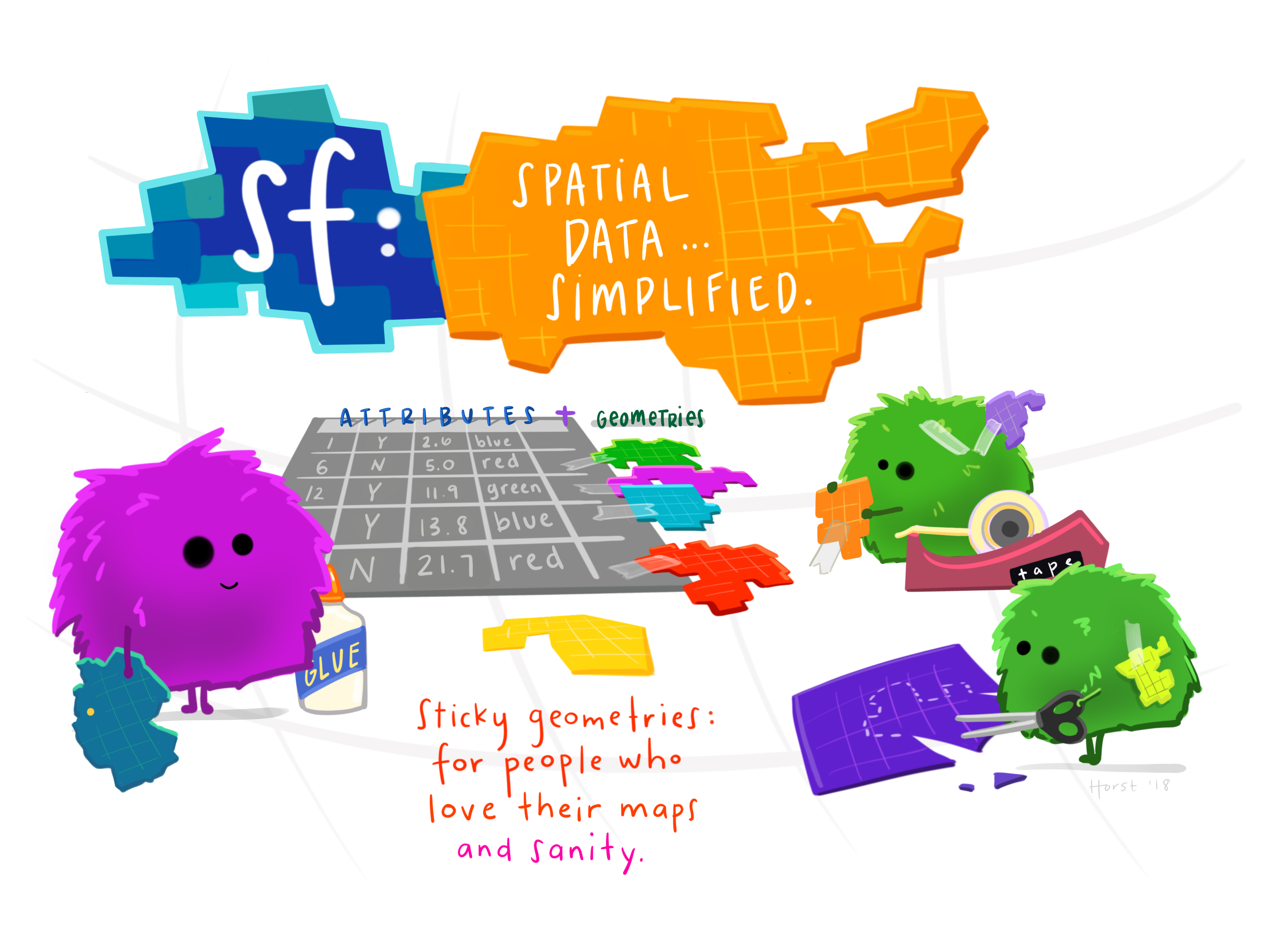
The sf library is a key tool for reading in, managing, and working with spatial data in R. sf stands for simple features (not San Francisco you Bay Area folks) and denotes a way to describe the spatial attributes of real life objects. The R object you will be working with most frequently for mapping is an sf dataframe. An sf dataframe is essentially a regular R dataframe, with a couple of extra features for use in mapping. These extra features exclusive to sf dataframes include:
sticky geometry columns
attached coordinate reference systems
some other spatial metadata
The most important of the above list is the sticky geometry column, which is a magical column that contains all of the geographic information for each row of data. Say for example you had a sf dataframe of all DC census tracts. Then the geometry column would contain all of the geographic points used to define DC census tract polygons. The stickiness of this column means that no matter what data munging/filtering you do, you will not be able to drop or delete the geometry column. Below is a graphic to help you understand this:
credits: @allisonhorst
This is what an sf dataframe looks like in the console:
# Read in spatial data about DC parks from DC Open Data Portaldc_parks <-st_read("https://opendata.arcgis.com/api/v3/datasets/287eaa2ecbff4d699762bbc6795ffdca_9/downloads/data?format=geojson&spatialRefId=4326",quiet =TRUE)# dc_parks <- st_read("mapping/data/dc_parks.geojson")# Select just a few columns for readabilitydc_parks <- dc_parks %>%select(NAME, geometry)# Print to the consoledc_parks
Simple feature collection with 256 features and 1 field
Geometry type: MULTIPOLYGON
Dimension: XY
Bounding box: xmin: -77.11113 ymin: 38.81718 xmax: -76.91108 ymax: 38.98811
Geodetic CRS: WGS 84
First 10 features:
NAME geometry
1 Plymouth Circle MULTIPOLYGON (((-77.04677 3...
2 Triangle Park RES 0566 MULTIPOLYGON (((-77.04481 3...
3 Shepherd Field MULTIPOLYGON (((-77.03528 3...
4 Marvin Caplan Memorial Park MULTIPOLYGON (((-77.03027 3...
5 Pinehurst Circle MULTIPOLYGON (((-77.06643 3...
6 Triangle Park 3278 0801 MULTIPOLYGON (((-77.01759 3...
7 Fort Stevens MULTIPOLYGON (((-77.02988 3...
8 Takoma Recreation Center MULTIPOLYGON (((-77.01794 3...
9 Takoma Community Center MULTIPOLYGON (((-77.01716 3...
10 Triangle Park RES 0648 MULTIPOLYGON (((-77.03362 3...
Note that there is some spatial metadata such as the Geometry Type, Bounding Box, and CRS which shows up as a header before the actual contents of the dataframe.
Since sf dataframes operate similarly to regular dataframes, we can use all our familiar tidyverse functions for data wrangling, including select, filter, rename, mutate, group_by and summarize. The sf package also has many functions that provide easy ways to replicate common tasks done in other GIS software like spatial joins, clipping, and buffering. Almost all of the mapping and geospatial analysis methods described in this guide rely on you having an sf dataframe. So let’s talk about how to get one!
Importing spatial data
Getting an sf dataframe is always the first step in the geospatial workflow. Here’s how to import spatial data for…
States and counties
We highly recommend using the library(urbnmapr) package, which was created by folks here at Urban to easily create state and county level maps. The get_urbn_map() function in the package allows you to read in spatial data on states and counties, with options to include territories. Importantly, it will also display AL and HI as insets on the map in accordance with the Urban Institute Data Visualization Style Guide. For information on how to install urbnmapr, see the GitHub repository.
Below is an example of how you would use urbnmapr to get an sf dataframe of all the states or counties in the US.
library(urbnmapr)# Get state datastates <-get_urbn_map("states", sf =TRUE)# Can also get county datacounties <-get_urbn_map("counties", sf =TRUE)
Other Census geographies
Use the library(tigris) package, which allows you to easily download TIGER and other cartographic boundaries from the US Census Bureau. In order to automatically load in the boundaries as sf objects, run once per R session.
library(tigris) has all the standard census geographies, including census tracts, counties, CBSAs, ZCTAs, congressional districts, tribal areas, and more. It also includes other elements such as water, roads, and military bases.
By default, libraray(tigris) will download large very large and detailed TIGER line boundary files. For thematic mapping, the smaller cartographic boundary files are a better choice, as they are clipped to the shoreline, generalized, and therefore usually smaller in size without losing too much accuracy. To load cartographic boundaries, use the cb = TRUE argument. If you are doing detailed geospatial analysis and need the most detailed shapefiles, then you should use the detailed TIGER line boundary files and set cb = FALSE.
Below is an example of how you would use library(tigris) to get a sf dataframe of all Census tracts in DC for 2019.
library(tigris)# Only need to set once per scriptoptions(tigris_class ="sf")dc_tracts <-tracts(state ="DC",cb =TRUE,year =2019)
Unlike library(urbnmapr), different functions are used to get geographic data for different geographic levels. For instance, the blocks() function will load census block group data, and the tracts() function will load tract data. Other functions include block_groups(), zctas() , and core_based_statistical_areas(). For the full list of supported geographies and functions, see the package vignette.
For folks interested in pulling in Census demographic information along with Census geographies, we recommend checking out the sister package to library(tigris): library(tidycensus). That package allows you to download in Census variables and Census geographic data simultaneously.
Countries
We recommend using the library(rnaturalearth) package, which is similar to library(tigris) but allows you to download and use boundaries beyond the US. Instead of setting class to sf one time per session as we did with library(tigris), you must set the returnclass = "sf" argument each time you use a function from the package. Below is an example of downloading in an sf dataframe of all the countries in the world.
Shapefiles and GeoJSONs are 2 common spatial file formats you will found out in the wild. library(sf) has a function called st_read which allows you to easily read in these files as sf dataframes. The only required argument is dsn or data source name. This is the filepath of the .shp file or the .geojson file on your local computer. For geojsons, dsn can also be a URL.
Below is an example of reading in a shapefile of fire stations in DC which is stored in mapping/data/shapefiles/. Note that shapefiles are actually stored as 6+ different files inside a folder. You need to provide the filepath to the file ending in .shp.
library(sf)# Print out all files in the directorylist.files("mapping/data/shapefiles")
# Read in .shp filedc_firestations <-st_read(dsn ="mapping/data/shapefiles/Fire_Stations.shp",quiet =TRUE)
And now dc_firestations is an sf dataframe you can use for all your mapping needs! st_read supports reading in a wide variety of other spatial file formats, including geodatabases, KML files, and over 200 others. For an incomplete list, please see the this sfvignette.
CSVs or dataframes with lat/lons
If you have a CSV with geographic information stored in columns, you will need to read in the CSV as a regular R dataframe and then convert to an sf dataframe. library(sf) contains the st_as_sf() function for converting regular R dataframes into an sf dataframe. The two arguments you must specify for this function are:
coords: A length 2 vector with the names of the columns corresponding to longitude and latitude (in that order!). For example, c("lon", "lat").
crs: The CRS (coordinate references system) for your longitude/latitude coordinates. Remember you need to specify both the
authority and the SRID code, for example (“EPSG:4326”). For more information on finding and setting CRS codes, please see the CRS section.
Below is an example of reading in data from a CSV and converting it to an sf dataframe.
library(sf)# Read in dataset of state capitals which is stored as a csvstate_capitals <-read_csv("mapping/data/state-capitals.csv")state_capitals <- state_capitals %>%# Specify names of the lon/lat columns in the CSV to use to make geometry colst_as_sf(coords =c("longitude", "latitude"),crs =4326 )
One common mistake is that before converting to an sf dataframe, you must drop any rows that have NA values for latitude or longitude. If your data contains NA values, then the st_as_sf() function will throw an error.
Appending spatial info to your data
Oftentimes, the data you are working with will just have state or county identifiers - like FIPS codes or state abbreviations - but will not contain any geographic information. In this case, you must do the extra work of downloading in the geographic data as an sf dataframe and then joining your non-spatial data to the spatial data. Generally this involves 3 steps:
Reading in your own data as a data frame
Reading in the geographic data as an sf dataframe
Using left_join to merge the geographic data with your own non spatial data and create a new expanded sf dataframe
Let’s say we had a dataframe on CHIP enrollment by state with state abbreviations.
# read the state CHIP datachip_by_state <-read_csv("mapping/data/chip-enrollment.csv") %>%# clean column names so there are no random spaces/uppercase letters janitor::clean_names()# print to the consolechip_by_state %>%head()
# A tibble: 6 × 3
state chip_enrollment state_abbreviation
<chr> <dbl> <chr>
1 Alabama 150040 AL
2 Alaska 15662 AK
3 Arizona 88224 AZ
4 Arkansas 120863 AR
5 California 2022213 CA
6 Colorado 167227 CO
In order to convert this to an sf dataframe, we need to read in the spatial boundaries for each state and append it to our dataframe. Here is how we do that with get_urbn_map() and left_join() .
library(urbnmapr)# read in state geographic data from urbnmaprstates <-get_urbn_map(map ="states", sf =TRUE)# left join state geographies to chip datachip_with_geographies <- states %>%left_join( chip_by_state,# Specify join column, which are slightly differently named in states and chip# respectivelyby =c("state_abbv"="state_abbreviation") )chip_with_geographies %>%select(state_fips, state_abbv, chip_enrollment)
Simple feature collection with 51 features and 3 fields
Geometry type: MULTIPOLYGON
Dimension: XY
Bounding box: xmin: -2600000 ymin: -2363000 xmax: 2516374 ymax: 732352.2
Projected CRS: NAD27 / US National Atlas Equal Area
First 10 features:
state_fips state_abbv chip_enrollment geometry
1 01 AL 150040 MULTIPOLYGON (((1150023 -15...
2 04 AZ 88224 MULTIPOLYGON (((-1386136 -1...
3 08 CO 167227 MULTIPOLYGON (((-786661.9 -...
4 09 CT 25551 MULTIPOLYGON (((2156197 -83...
5 12 FL 374884 MULTIPOLYGON (((1953691 -20...
6 13 GA 232050 MULTIPOLYGON (((1308636 -10...
7 16 ID 35964 MULTIPOLYGON (((-1357097 78...
8 18 IN 114927 MULTIPOLYGON (((1042064 -71...
9 20 KS 79319 MULTIPOLYGON (((-174904.2 -...
10 22 LA 161565 MULTIPOLYGON (((1075669 -15...
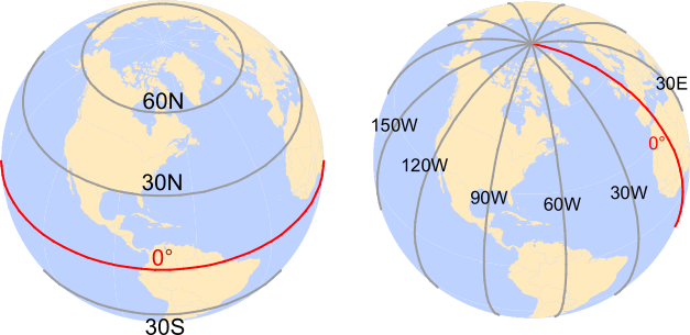
All spatial data has a CRS, which specifies how to identify a location on earth.
It’s important that all spatial datasets you are working with be in the same CRS. You can find the CRS with st_crs() and change the CRS with st_transform().
The Urban Institute Style Guide requires the use of the Atlas Equal Earth Projection ("ESRI:102003") for national maps. For state and local maps, use this handy guide to find an appropriate State Plane projection.
The long version
Coordinate reference systems (CRS) specify the 3d shape of the earth and optionally how we project that 3d shape onto a 2d surface. They are an important part of working with spatial data as you need to ensure that all the data you are working with are in the same CRS in order for spatial operations and maps to be accurate.
CRS can be specified either by name (ie Maryland State Plane) or Spatial Reference System IDentifier (SRID). THe SRID is a numeric identifier that uniquely identifies a coordinate reference system. Generally when referring to an SRID, you need to refer to an authority (ie the data source) and a unique ID. An example is EPSG:26985 which refers to the Maryland State plane projection from the EPSG, or ESRI:102003 which refers to the Atlas Equal Area projection from ESRI. Most CRS codes will be from the EPSG, and some from ESRI and others. A good resource for finding/validating CRS codes is epsg.io.
Sidenote - EPSG stands for the now defunct European Petroleum Survey Group. And while oil companies have generally been terrible for the earth, the one nice thing they did for the earth was to set up common standards for coordinate reference systems.
You might be thinking well isn’t the earth just a sphere? Why do we need all this complicated stuff? And the answer is well the earth is kind of a sphere, but it’s really more of a misshapen ellipsoid which is pudgier at the equator than at the poles. To visualize how coordinate reference systems work, imagine that the earth is a (lumpy) orange. Now peel the skin off an orange and try to flatten it. There are many ways to do it, but all will create distortions of some kind. The CRS will give us the formula we’ve used to specify the shape of the orange (usually a sphere or ellipsoid of some kind) and optionally, specify how we flattened the orange into 2d.
Broadly, there are two kinds of Coordinate Reference Systems:
projection: mathematical formula used to convert a 3d coordinate system to a 2d flat coordinate system
Many different kinds of projections, including Equal Area, Equidistant, Conformal, etc
All projections distort the true shape of the earth in some way, either in terms of shape, area, or angle. Required xkcd comic
Usually use linear units (ie feet, meters) and therefore useful for distance based spatial operations (ie creating buffers)
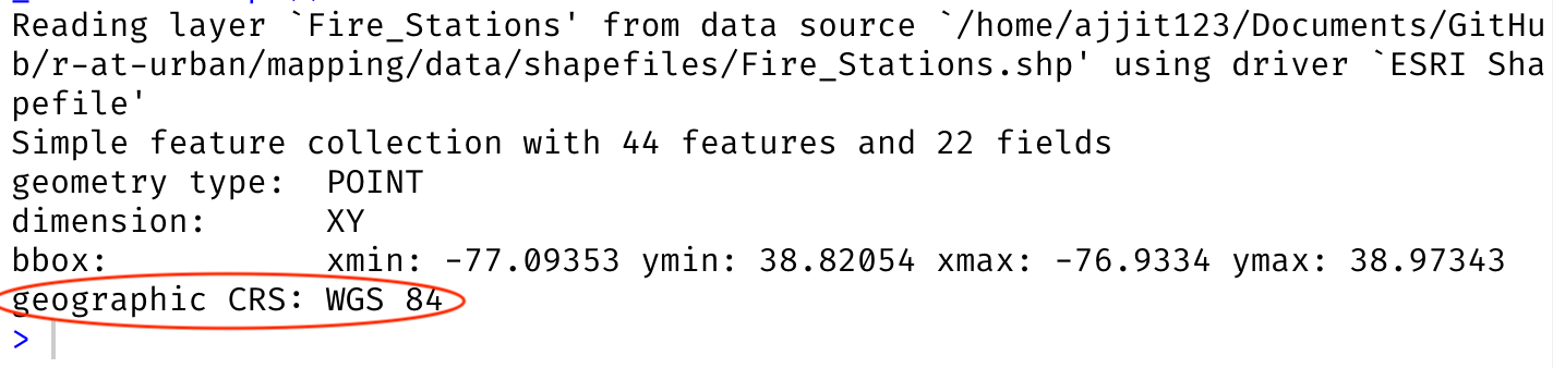
Finding the CRS
If you are lucky, your data will have embedded CRS data that will be automatically detected when the file is read in. This is usually the case for GeoJSONS (.geojson) and shapefiles (.shp). When you use st_read() on these files, you should see the CRS displayed in the metadata:
You can also the st_crs() function to find the CRS. The CRS code is located at the end in ID[authority, SRID].
Sometimes, the CRS will be blank or NA as the dataset did not specify the CRS. In that case you MUST find and set the CRS for your data before proceeding with analysis. Below are some good rules of thumb for finding out what the CRS for your data is:
For geojsons, the CRS should always be EPSG:4326 (or WGS 84). The official geojson specification states that this is the only valid CRS for geojsons, but in the wild, this may not be true 100% of the time.
For shapefiles, there should be a file that ends in .proj in the same directory as the .shp file. This file contains the projection information for that file and should be used automatically when reading in shapefiles.
For CSV’s with latitude/longitude columns, the CRS is usually EPSG:4326 (or WGS 84).
Look at the metadata and any accompanying documentation to see if the coordinate reference system for the data is specified
If none of the above rules of thumb apply to you, check out the crsuggest R package.
Once you’ve identified the appropriate CRS, you can set the CRS for your data with st_crs():
# If you are certain that your data contains coordinates in the ESRI Atlas Equal Earth projectionsst_crs(some_sf_dataframe) <-st_crs("ESRI:102003")
Transforming the CRS
Often you will need to change the CRS for your sf dataframe so that all datasets you are using have the same CRS, or to use a projected CRS for performing more accurate spatial operations. You can do this with st_transform:
# Transforming CRS from WGS 84 to Urban required Equal Earth Projectionstate_capitals <- state_capitals %>%st_transform("ESRI:102003")
st_transform() also allows you to just use the CRS of another sf dataframe when transforming.
# transform CRS of chip_with_geographies to be the same as CRS of dc_firestationschip_with_geographies <- chip_with_geographies %>%st_transform(crs =st_crs(state_capitals))
If you are working with local data, you should use an appropriate state plane projection instead of the Atlas Equal Earth projection which is meant for national maps. library(crsuggest) can simplify the process of picking an appropriate state plane CRS.
library(crsuggest)suggest_crs(dc_firestations) %>%# Use the value in the "crs_code" column to transform CRS'shead(4)
In order to start mapping, you need an sf dataframe. If you don’t have one, see the Get Spatial Data section above.
The basics
library(ggplot2)
Most mapping in R fits the same theoretical framework as plotting in R using library(ggplot2). To learn more about ggplot2, visit the Data Viz page or read the official ggplot book.
The key function for mapping is the special geom_sf() function which works with sf dataframes. This function magically detects whether you have point or polygon spatial data and displays the results on a map.
A simple map
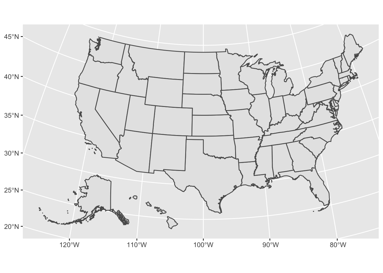
To make a simple map, add geom_sf() to a ggplot() and set data = an_sf_dataframe. Below is code for making a map of all 50 states using library(urbnmapr):
library(urbnmapr)states <-get_urbn_map("states", sf =TRUE)ggplot() +geom_sf(data = states,mapping =aes() )
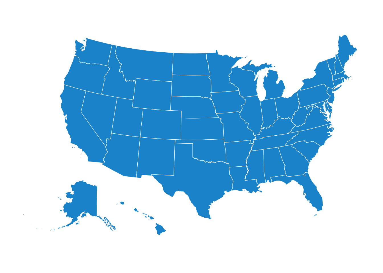
Styling
library(urbnthemes)
library(urbnthemes) automatically styles maps in accordance with the Urban Institute Data Visualization Style Guide. By using library(urbnthemes), you can create publication ready maps you can immediately drop in to Urban research briefs or blog posts.
To install urbnthemes, visit the package’s GitHub repository and follow the instructions. There are 2 ways to use the urbnthemes functions:
library(urbnthemes)# You can either run this once per script to automatically style all maps with# the Urban themeset_urbn_defaults(style ="map")# Or you can add `+ theme_urbn_map()` to the end of every map you makeggplot() +geom_sf(states, mapping =aes()) +theme_urbn_map()
Layering
You can layer multiple points/lines/polygons on top of each other using the + operator from library(ggplot2). The shapes will appear from bottom to top (ie the last mapped object will show up on top). It is important that all layers are in the same CRS (coordinate reference system).
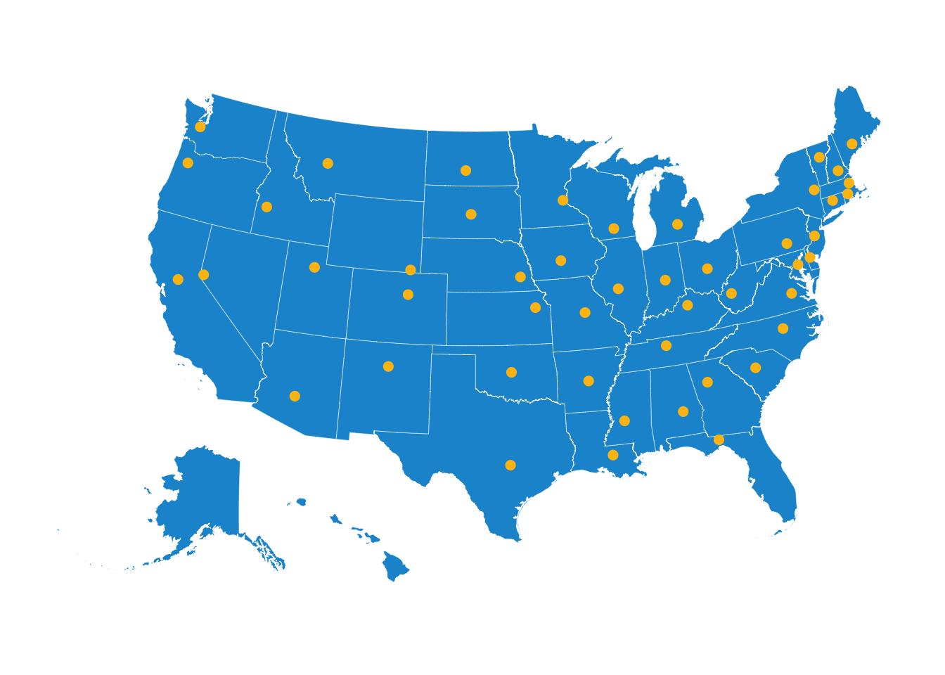
state_capitals <- state_capitals %>%# This will change CRS to ESRI:102003 and shift the AK and HI state capitals# point locations to the appropriate locations on the inset maps. tigris::shift_geometry() %>%# For now filter out AL and HI as their state capitals will be slightly off.filter(!state %in%c("Alaska", "Hawaii"))ggplot() +geom_sf(data = states,mapping =aes() ) +# Note we change the data argumentgeom_sf(data = state_capitals,mapping =aes(),# urbnthemes library has urbn color palettes built in.color = palette_urbn_main["yellow"],size =2.0 ) +theme_urbn_map()
Fill and Outline Colors
The same commands used to change colors, opacity, lines, size, etc. in charts can be used for maps too. To change the colors of the map , just use the fill = and color = parameters in geom_sf(). fill will change the fill color of polygons; color will change the color of polygon outlines, lines, and points.
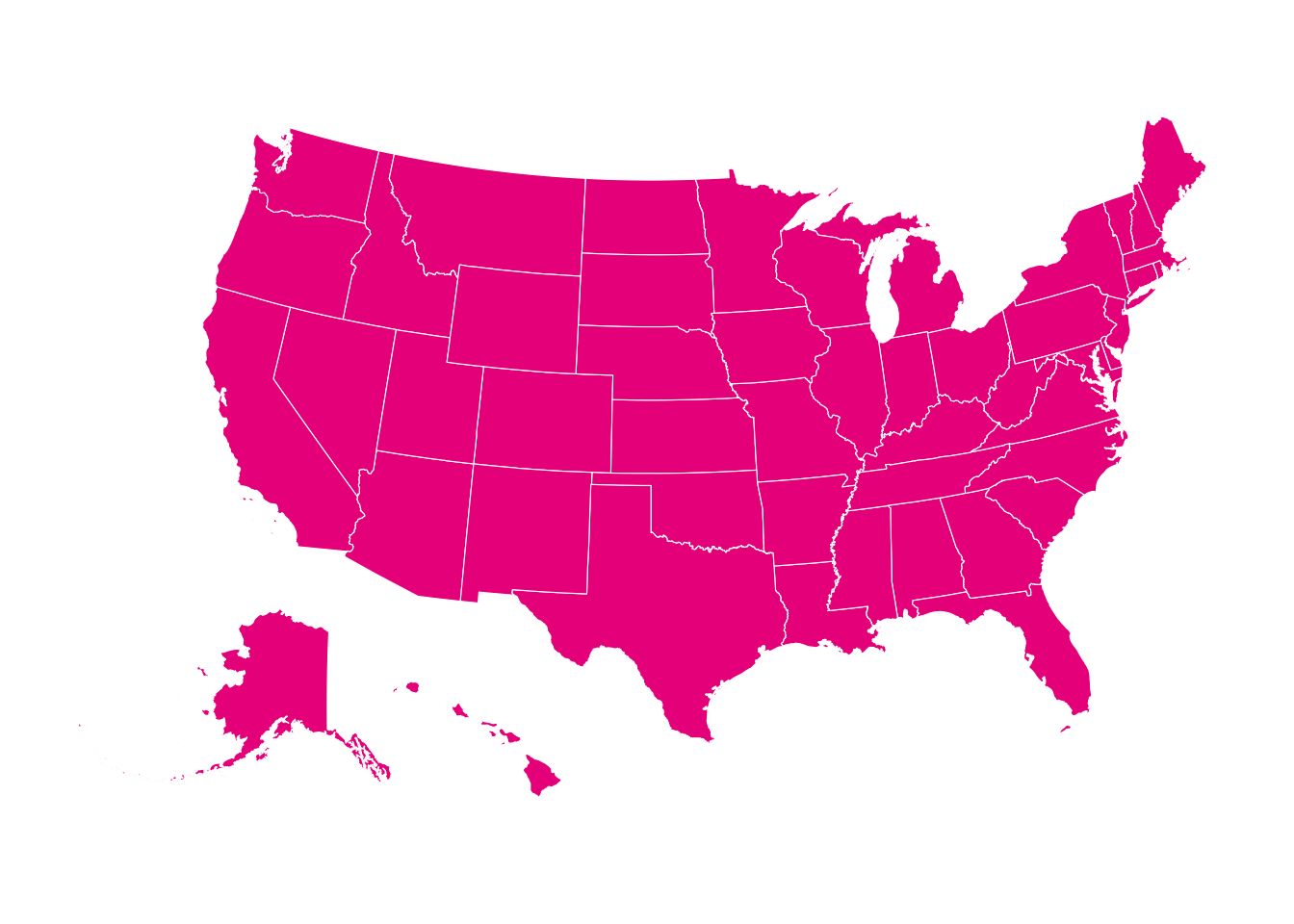
Generally, maps that show the magnitude of a variable use the blue sequential ramp and maps that display positives and negatives use the diverging color ramp.library(urbnthemes) contains inbuilt. helper variables (like palette_urbn_main) for accessing color palettes from the Urban Data Viz Style guide. If for example you want states to be Urban’s magenta color:
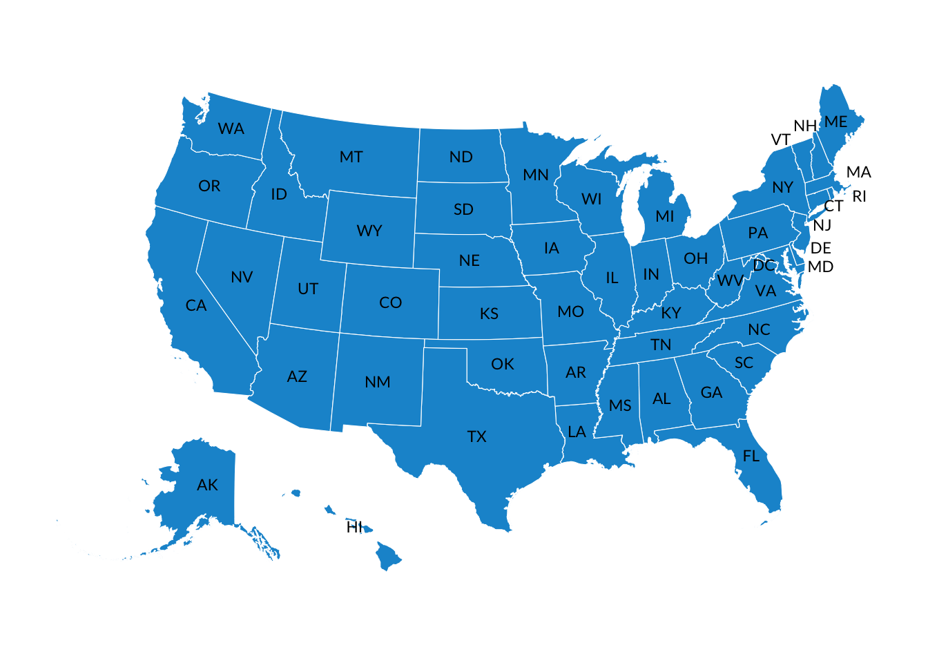
You can also add text, like state abbreviations, directly to your map using geom_sf_text and the helper function get_urbn_labels().
library(urbnmapr)ggplot() +geom_sf(states,mapping =aes(),color ="white" ) +theme_urbn_map() +# Generates dataframe of state abbv and appropriate location to plot themgeom_sf_text(data =get_urbn_labels(map ="states",sf =TRUE ),aes(label = state_abbv),size =3 )
There’s also geom_sf_label() if you want labels with a border.
Map Gallery
Below are copy and pasteable examples of maps you can make, after you have an sf dataframe.
Choropleth Maps
Choropleth maps display geographic areas with shades, colors, or patterns in proportion to a variable or variables. Choropleth maps can represent massive geographies like the entire world and small geographies like Census Tracts. To make a choropleth map, you need to set geom_sf(aes(fill = some_variable_name)). Below are examples
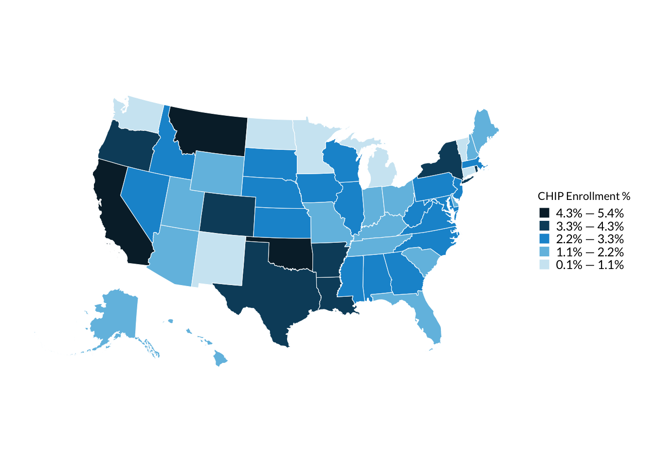
Continuous color scale
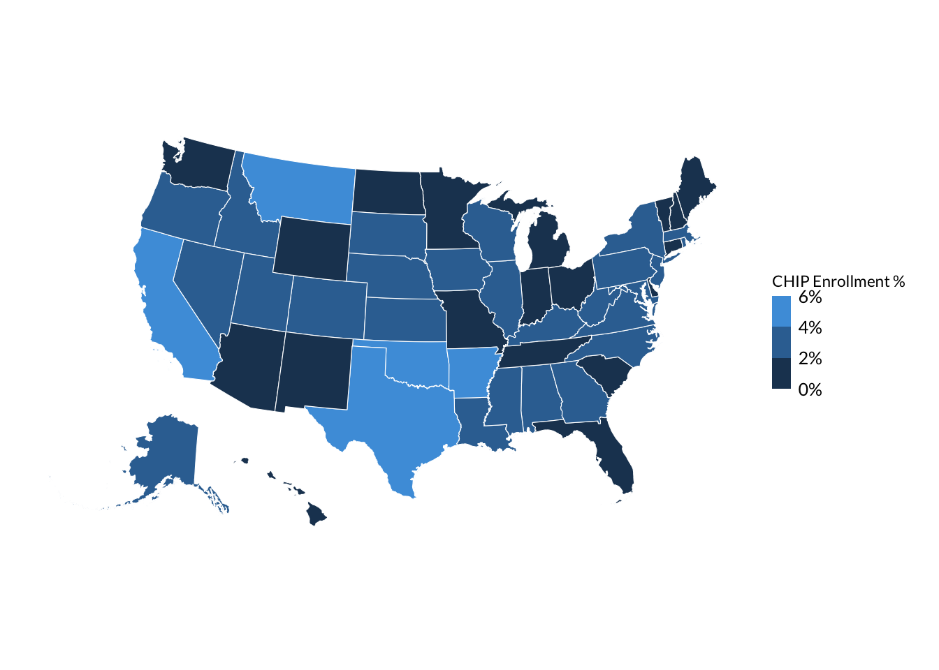
# Map of CHIP enrollment percentage by statechip_with_geographies_map <- chip_with_geographies %>%ggplot() +geom_sf(aes(# Color in states by the chip_pct variablefill = chip_pct ))# Below add-ons to the map are optional, but make the map look prettier.chip_with_geographies_map +# scale_fill_gradientn adds colors with more interpolation and reverses color scalescale_fill_gradientn(# Convert legend from decimal to percentageslabels = scales::percent_format(),# Make legend title more readablename ="CHIP Enrollment %",# Manually add 0 to lower limit to include it in legend. NA=use maximum value in datalimits =c(0, NA),# Set number of breaks on legend = 3n.breaks =3 )
Discrete color scale
The quick and dirty way is with scale_fill_steps(), which creates discretized bins for continuous variables:
chip_with_geographies %>%ggplot() +geom_sf(aes(# Color in states by the chip_pct variablefill = chip_pct )) +scale_fill_steps(# Convert legend from decimal to percentageslabels = scales::percent_format(),# Make legend title more readablename ="CHIP Enrollment %",# Show top and bottom limits on legendshow.limits =TRUE,# Roughly set number of bins. Won't be exact as R uses algorithms under the# hood for pretty looking breaks.n.breaks =4 )
Often you will want to manually generate the bins yourself to give you more fine grained control over the exact legend text. (ie 1% - 1.8%, 1.8 - 2.5%, etc). Below is an example of discretizing the continuous chip_pct variable yourself using cut_interval() and a helper function to get nice looking interval labels:
# Helper function to clean up R generated intervals into nice looking interval labelsformat_interval <-function(interval_text) { text <- interval_text %>%# Remove open and close brackets which is R generated math notationstr_remove_all("\\(") %>%str_remove_all("\\)") %>%str_remove_all("\\[") %>%str_remove_all("\\]") %>%str_replace_all(",", " — ")# Convert decimal ranges to percent ranges text <- text %>%str_split(" — ") %>%map(~as.numeric(.x) %>% scales::percent() %>%paste0(collapse =" — ")) %>%unlist() %>%# By default character vectors are plotted in alphabetical order. We want# factors in reverse alphabetical order to get correct colors in ggplotfct_rev()return(text)}chip_with_geographies <- chip_with_geographies %>%# cut_interval into n groups with equal range. Set boundary so 0 is included in the binsmutate(chip_pct_interval =cut_interval(chip_pct, n =5)) %>%# Generate nice looking interval labelsmutate(chip_pct_interval =format_interval(chip_pct_interval))
And now we can map the discretized chip_pct_interval variable using geom_sf():
chip_with_geographies %>%ggplot() +geom_sf(aes(# Color in states by the chip_pct variablefill = chip_pct_interval )) +# Default is to use main urban palette, which assumes unrelated groups. We# adjust colors manually to be on Urban cyan palettescale_fill_manual(values = palette_urbn_cyan[c(8, 7, 5, 3, 1)],name ="CHIP Enrollment %" )
In addition to cut_interval there are similar functions for creating intervals/bins with slightly different rules. When creating bins, be careful as changing the number of bins can drastically change how the map looks.
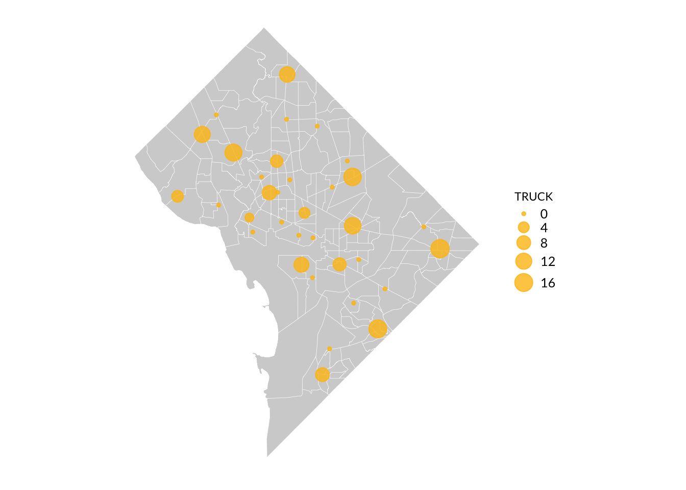
Bubble Maps
This is just a layered map with one polygon layer and one point layer, where the points are sized in accordance with a variable in your data.
set_urbn_defaults(style ="map")# Get sf dataframe of DC tractslibrary(tigris)dc_tracts <-tracts(state ="DC",year =2019,progress_bar =FALSE)# Add bubbles for firestationsggplot() +geom_sf(data = dc_tracts, fill = palette_urbn_main["gray"]) +geom_sf(data = dc_firestations,# Size bubbles by number of trucks at each stationaes(size = TRUCK),color = palette_urbn_main["yellow"],# Adjust transparency for readabilityalpha =0.8 )
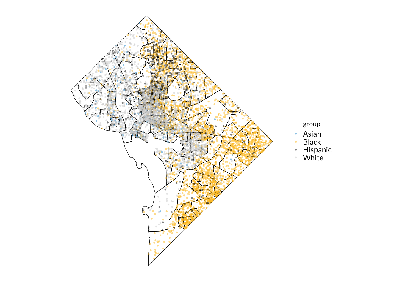
Dot-density Maps
These maps scatter dots within a geographic area. Typically each dot represents a unit (like 100 people, or 1000 houses). To create this kind of map, you need to start with an sf dataframe that is of geometry type POLYGON or MULTIPOLYGON and then sample points within the polygon.
The below code generates a dot-density map representing people of different races within Washington DC tracts The code may look a little complicated, but the key workhorse function is st_sample() which samples points within each polygon to use in the dot density map:
library(tidycensus)# Get counts by race of DC tractsdc_pop <-get_acs(geography ="tract",state ="DC",year =2019,variables =c(Hispanic ="DP05_0071",White ="DP05_0077",Black ="DP05_0078",Asian ="DP05_0080" ),geometry =TRUE,progress_bar =FALSE)# Get unique groups (ie races)groups <-unique(dc_pop$variable)# For each unique group (ie race), generate sampled pointsdc_race_dots <-map_dfr(groups, ~ { dc_pop %>%# .x = the group used in the loopfilter(variable == .x) %>%# Use the projected MD state plane for accuracyst_transform(crs ="EPSG:6487") %>%# Have every dot represent 100 peoplemutate(est100 =as.integer(estimate /100)) %>%st_sample(size = .$est100, exact =TRUE) %>%st_sf() %>%# Add group (ie race) as a column so we can use it when plottingmutate(group = .x)})ggplot() +# Plot tracts, then dots on top of tractsgeom_sf(data = dc_pop,# Make interior of tracts transparent and boundaries blackfill ="transparent",color ="black" ) +geom_sf(data = dc_race_dots,# Color in dots by racial groupaes(color = group),# Adjust transparency and size to be more readablealpha =0.5,size =1.1,stroke =FALSE )
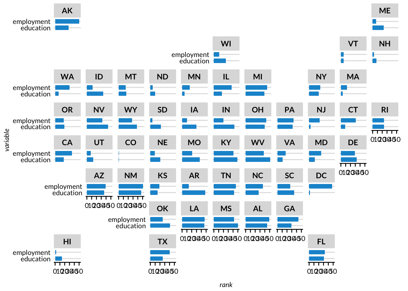
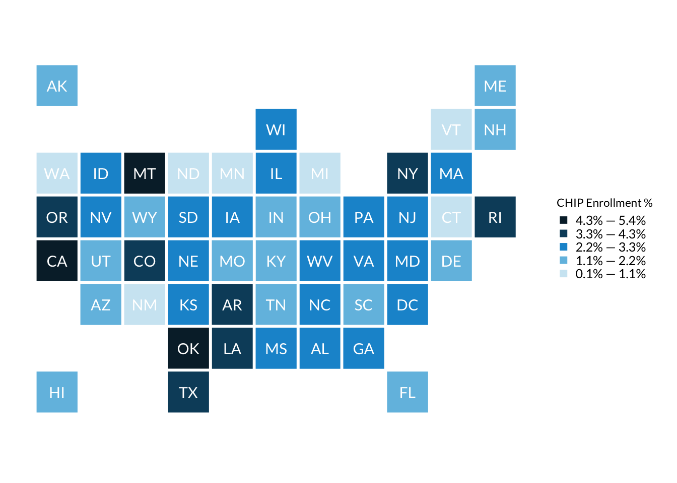
Geofacets
Geofaceting arranges sub-geography-specific plots into a grid that resembles a larger geography (usually the US). This can be a useful alternative to choropleth maps, which tend to overemphasize low-population density areas with large areas. To make geofacetted charts, use the facet_geo() function from the geofacet library, which can be thought of as equivalent to ggplot2’s facet_wrap(). For this example, we’ll use the built-in state_ranks data.
library(geofacet)head(state_ranks %>%as_tibble())
# A tibble: 6 × 4
state name variable rank
<chr> <chr> <chr> <dbl>
1 AK Alaska education 28
2 AK Alaska employment 50
3 AK Alaska health 25
4 AK Alaska wealth 5
5 AK Alaska sleep 27
6 AK Alaska insured 50
set_urbn_defaults(style ="print")state_ranks %>%filter(variable %in%c("education", "employment")) %>%ggplot(aes(x = rank, y = variable)) +geom_col() +facet_geo(facets ="state",# Use custom urban geofacet grid which is built into urbnthemes# For now we need to rename a few columns as urbnthemes has to be# updatedgrid = urbnthemes::urbn_geofacet %>%rename(code = state_code,name = state_name ) )
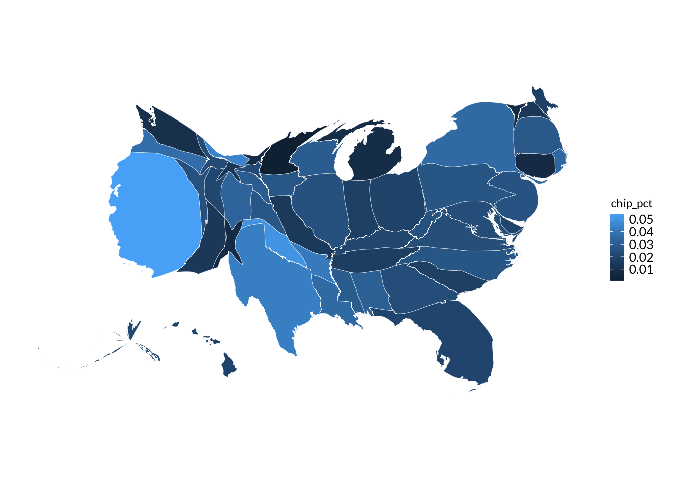
Cartograms are a modified form of a choropleth map with intentionally distorted sizes that map to a variable in your data. Below we create a cartogram with library(cartogram) where the state sizes are proportional to the population.
library(cartogram)set_urbn_defaults(style ="map")chip_with_geographies_weighted <- chip_with_geographies %>%# Note column name needs to be in quotes for this packagecartogram_cont(weight ="population")ggplot() +geom_sf(data = chip_with_geographies_weighted,# Color in states by chip percentagesaes(fill = chip_pct) )
Interactive Maps
Interactive maps can be a great exploratory tool to explore and understand your data. And luckily there are a lot of new R packages that make it really easy to create them. Interactive maps are powerful but we do not recommend them for official use in Urban publications as getting them in Urban styles and appropriate basemaps can be tricky (reach out to anarayanan@urban.org if you really want to include them).
library(mapview)
library(mapview) is probably the most user friendly of the interactive mapping R libraries. All you have to do to create an interactive map is:
library(mapview)chip_with_geographies_for_interactive_mapping <- chip_with_geographies %>%# Filter out AL and HI bc they would appear in Mexico. If you want AL, HI and# in the correct place in interactive maps, make sure to use tigris::states()filter(!state_abbv %in%c("AK", "HI"))mapview(chip_with_geographies_for_interactive_mapping)
When you click on an object, you get a popup table of all it’s attributes. And when you hover over an object, you get a popup with an object id.
Each of the above behaviors can be changed if desired. As you’ll see in the below section, the syntax for library(mapview) is significantly different from library(ggplot2) so be careful!
Coloring in points/polygons
In order to create a choropleth map where we color in the points/polygons by a variable, we need to feed in a column name in quotes to thezcol argument inside the mapview() function:
# Create interactive state map colored in by chip enrollmentmapview(chip_with_geographies_for_interactive_mapping, zcol ="chip_enrollment")
If you want more granular control over the color palette for the legend can also feed in a vector of color hex codes to col.regions along with a column name to zcol. This will create a continuous color range along the provided colors. Be careful though as the color interpolation is not perfect.
To learn more about more advanced options with mapview maps, check out the documentation page and the reference manual.
There are also other interactive map making packages in R like leaflet (which mapview is a more user friendly wrapper of), tmap, and mapdeck. To learn about these other packages, this book chapter is a good starting point.
Spatial Operations
Cropping
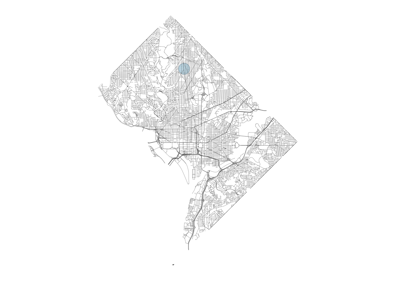
Cropping (or clipping) is geographically filtering an sf dataframe to just the area we are interested in. Say we wanted to look at the roads around Fire Station 24 in DC.
library(tigris)library(units)dc_firestations <- dc_firestations %>%st_transform("EPSG:6487")# Draw 500 meter circle around one fire stationfire_station_24_buffered <- dc_firestations %>%filter(NAME =="Engine 24 Station") %>%st_buffer(set_units(500, "meter"))# Get listing of all roads in DCdc_roads <-roads(state ="DC",county ="District of Columbia",class ="sf",progress_bar =FALSE) %>%st_transform("EPSG:6487")# View roads on top of fire_stationggplot() +# Order matters! We need to plot fire_stations first, and then roads on top# to see overlapping firestationsgeom_sf(data = fire_station_24_buffered,fill = palette_urbn_cyan[1],color = palette_urbn_cyan[7] ) +geom_sf(data = dc_roads,color = palette_urbn_gray[7] ) +theme_urbn_map()
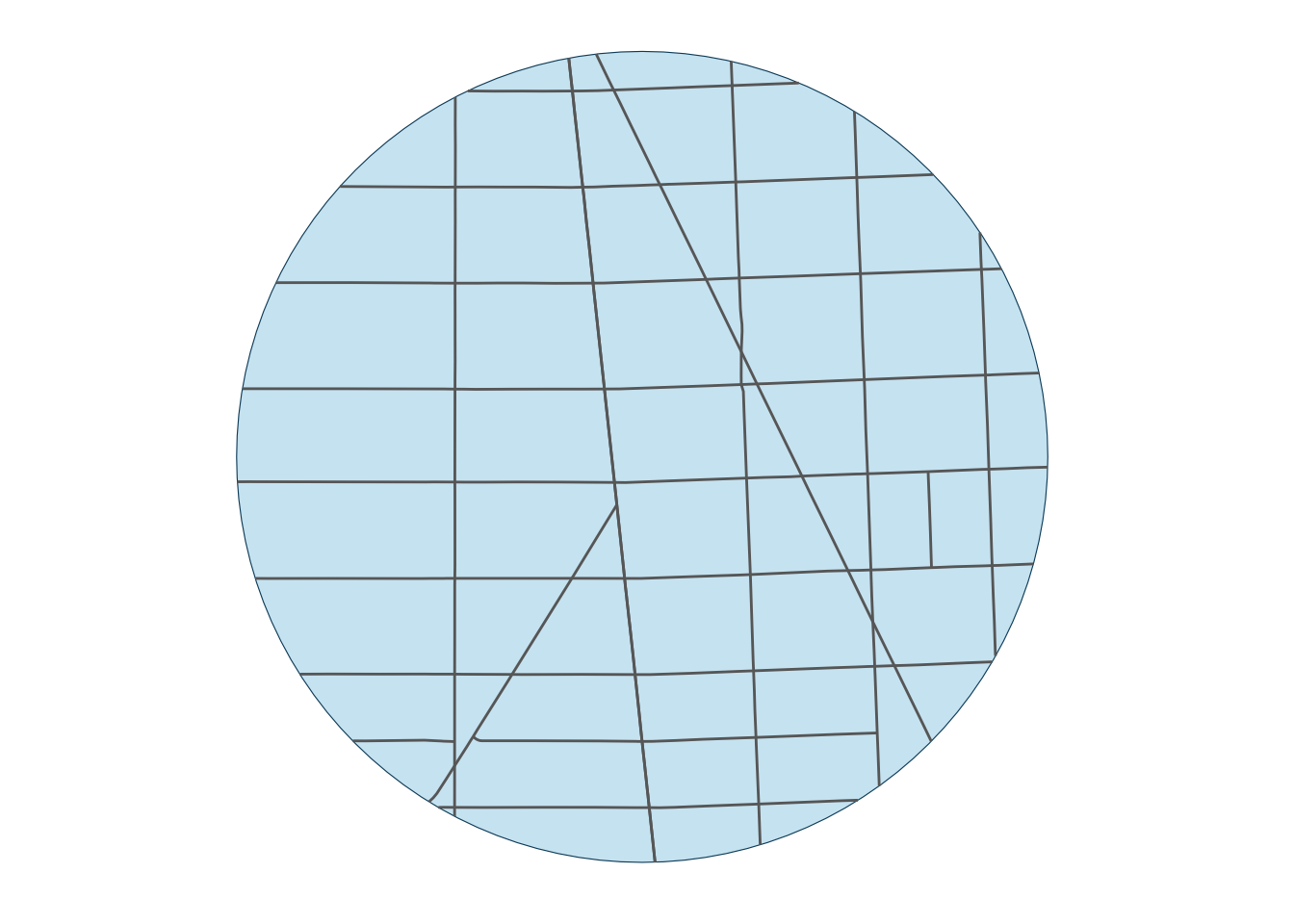
We can clip the larger roads dataframe to just roads that overlap with the circle around the fire station with st_intersection().
# Use st_intersection() to crop the roads data to just roads within the# fire_station radiusdc_roads_around_fire_station_24_buffered <- fire_station_24_buffered %>%st_intersection(dc_roads)ggplot() +geom_sf(data = fire_station_24_buffered,fill = palette_urbn_cyan[1],color = palette_urbn_cyan[7] ) +geom_sf(data = dc_roads_around_fire_station_24_buffered,color = palette_urbn_gray[7] ) +theme_urbn_map()
More Coming Soon!
Calculating Distance
Spatial Joins
Point to Polygon
Polygon to Polygon
Aggregating
Drive/Transit times
Geocoding
Geocoding is the process of turning text (usually addresses) into geographic coordinates (usually latitudes/longitudes) for use in mapping. For Urban researchers, we highly recommend using the Urban geocoder as it is fast, accurate, designed to work with sensitive/confidential data and most importantly free to use for Urban researchers! To learn about how we set up and chose the geocoder for the Urban Institute, you can read our Data@Urban blog.
Cleaning Addresses
The single most important factor in getting accurate geocoded data is having cleaned, well structured address data. This can prove difficult as address data out in the wild is often messy and unstandardized. While the rules for cleaning addresses are very data specific, below are some examples of clean addresses you should aim for in your data cleaning process:
f_address
Type of address
123 Troy Drive, Pillowtown, CO, 92432
residnetial address
789 Abed Avenue, Apt 666, Blankesburg, CO, 92489
residential apartment address
Shirley Boulevard and Britta Drive, Blanketsburg, CO, 92489
street intersection
Pillowtown, CO
city
92489, CO
Zip Code
All that being said, our geocoder is pretty tolerant of different address formats, typos/spelling errors and missing states, zip codes, etc. So don’t spend too much time cleaning every address in the data. Also note that while our geocoder is able to geocode cities and zip codes, it will return the lat/lon of the center of the city/zip code, which may not be what you want.
Generate a CSV with a column named f_address which contains the addresses in single line format (ie 123 Abed Avenue, Blanketsburg, CO, 94328). This means that if you have the addresses split across multiple columns (ie Address, City, State, Zip columns), you will need to concatenate them into one column. Also see our Address cleaning section above.
Go to the Urban geocoder and answer the initial questions. This will tell you whether your data is non-confidential or confidential data, and allow you to upload your CSV for geocoding.
Wait for an email telling you your results are ready. If your data is non-confidential, this email will contain a link to your geocoded results. This link expires in 24 hours, so make sure to download your data before then. If you data is confidential, the email will contain a link to the location on the Y Drive where your confidential geocoded data is stored. You can specify this output folder when submitting the CSV in step 1.
Geocoder outputs
The geocoded file will be your original data, plus a few more columns (including latitude and longitude). each of the new columns that have been appended to your original data. It’s very important that you take a look at the Addr_type column in the CSV before doing further analysis to check the accuracy of the geocoding process.
Column
Description
Match_addr
The actual address that the inputted address was matched to. This is the address that the geocoder used to get Latitudes / Longitudes. If there are potentially many typos or non standard address formats in your data file, you will want to take a close look at this column to confirm that the matched address correctly handled typos and badly formatted addresses.
Longitude
The WGS 84 datum Longitude (EPSG code 4326)
Latitude
The WGS 84 datum Latitude (EPSG code 4326)
Addr_type
The match level for a geocode request. This should be used as an indicator of the precision of geocode results. Generally, Subaddress, PointAddress, StreetAddress, and StreetInt represent accurate matches. The list below contains all possible values for this field. Green values represent High accuracy matches, yellow represents Medium accuracy matches and red represents Low accuracy/inaccurate matches. If you have many yellow and red values in your data, you should manually check the results before proceeding with analysis. All possible values:
Subaddress: A subset of a PointAddress that represents a house or building subaddress location, such as an apartment unit, floor, or individual building within a complex. The UnitName, UnitType, LevelName, LevelType, BldgName, and BldgType field values help to distinguish subaddresses which may be associated with the same PointAddress. Reference data consists of point features with associated house number, street name, and subaddress elements, along with administrative divisions and optional postal code; for example, 3836 Emerald Ave, Suite C, La Verne, CA, 91750.
PointAddress: A street address based on points that represent house and building locations. Typically, this is the most spatially accurate match level. Reference data contains address points with associated house numbers and street names, along with administrative divisions and optional postal code. The X / Y (Longitude/Latitude) and geometry output values for a PointAddress match represent the street entry location for the address; this is the location used for routing operations. The DisplayX and DisplayY values represent the rooftop, or actual, location of the address. Example: 380 New York St, Redlands, CA, 92373.
StreetAddress — A street address that differs from PointAddress because the house number is interpolated from a range of numbers. Reference data contains street center lines with house number ranges, along with administrative divisions and optional postal code information, for example, 647 Haight St, San Francisco, CA, 94117.
StreetInt: A street address consisting of a street intersection along with city and optional state and postal code information. This is derived from StreetAddress reference data, for example, Redlands Blvd & New York St, Redlands, CA, 92373.
StreetName: Similar to a street address but without the house number. Reference data contains street centerlines with associated street names (no numbered address ranges), along with administrative divisions and optional postal code, for example, W Olive Ave, Redlands, CA, 92373.
StreetAddressExt: An interpolated street address match that is returned when parameter matchOutOfRange=true and the input house number exceeds the house number range for the matched street segment.
DistanceMarker: A street address that represents the linear distance along a street, typically in kilometers or miles, from a designated origin location. Example: Carr 682 KM 4, Barceloneta, 00617.
PostalExt: A postal code with an additional extension, such as the United States Postal Service ZIP+4. Reference data is postal code points with extensions, for example, 90210-3841.
POI: —Points of interest. Reference data consists of administrative division place-names, businesses, landmarks, and geographic features, for example, Golden Gate Bridge.
Locality: A place-name representing a populated place. The Type output field provides more detailed information about the type of populated place. Possible Type values for Locality matches include Block, Sector, Neighborhood, District, City, MetroArea, County, State or Province, Territory, Country, and Zone. Example: Bogotá, COL,
PostalLoc: A combination of postal code and city name. Reference data is typically a union of postal boundaries and administrative (locality) boundaries, for example, 7132 Frauenkirchen.
Postal: Postal code. Reference data is postal code points, for example, 90210 USA.
Score
A number from 1–100 indicating the degree to which the input tokens in a geocoding request match the address components in a candidate record. A score of 100 represents a perfect match, while lower scores represent decreasing match accuracy.
Status
Indicates whether a batch geocode request results in a match, tie, or unmatched. Possible values include
M - Match. The returned address matches the input address and is the highest scoring candidate.
T - Tied. The returned address matches the input address but has the same score as one or more additional candidates.
U - Unmatched. No addresses match the inputted address.
geometry
The WKT (Well-known text) representation of the latitudes and longitudes. This column may be useful if you’re reading the CSV into R, Python, or ArcGIS
Region
The state that Match_addr is located in
RegionAbbr
Abbreviated State Name. For example, CA for California
Subregion
The county that the input address is located in
MetroArea
The name of the Metropolitan area that Match_addr is located in. This field may be blank if the input address is not located within a metro area.
City
The city that Match_addr is located in
Nbrhd
The Neighborhood that Match_addr is located in. Note these are ESRI defined neighborhoods which may or may not align with other sources neighborhood definitions

